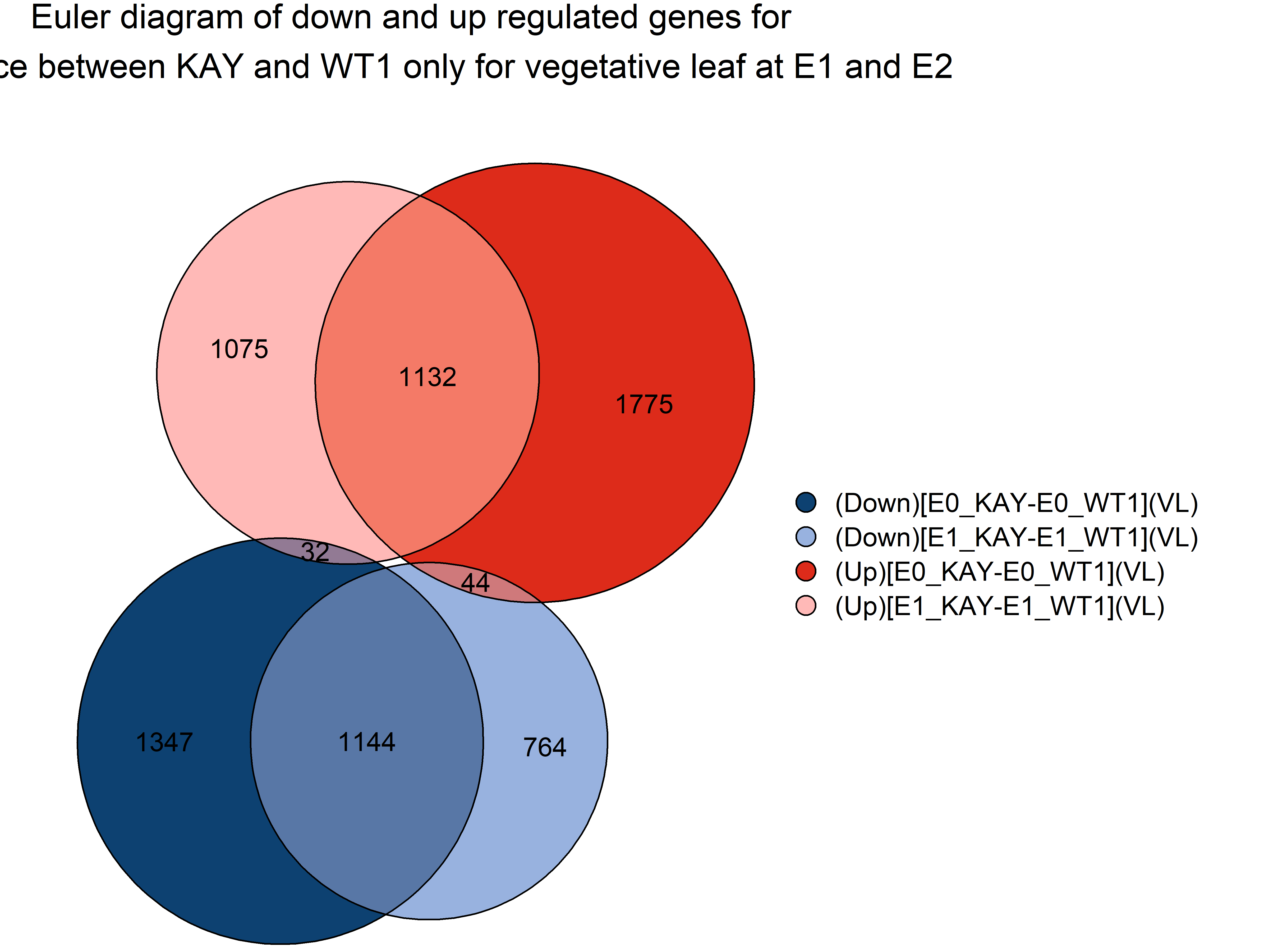
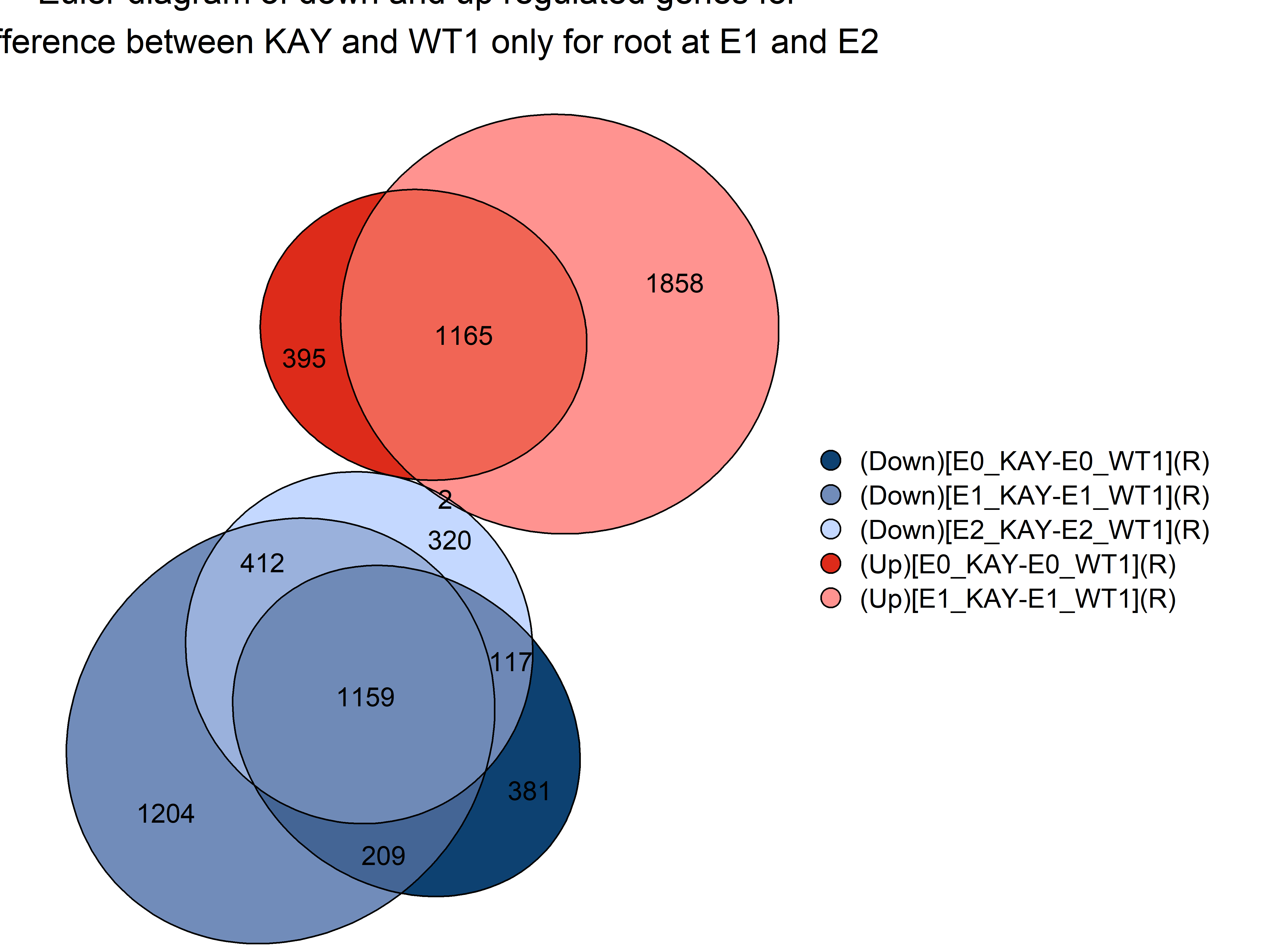
--- output: html_document editor_options: chunk_output_type: console --- ## KAY vs CAM before and during stress stage in roots and shoots for control condition ```{r} # pkg library (dplyr)library (factoextra)library (DESeq2) # BiocManager::install("DESeq2") library (readxl)library (tidyr)library (vsn) # for meanSdPlot #BiocManager::install("vsn") library (pheatmap)library (RColorBrewer)library (ggrepel)library (readxl)library (gridExtra)library (patchwork)library (ggrepel)library (mixOmics)library (colorspace)library (RColorBrewer)# for GO terme library (clusterProfiler)library (readxl)library (GO.db)library (AnnotationDbi) # BiocManager::install("AnnotationDbi") library (ggnewscale) # to have two scale_fill # src # src source (here:: here ("src/function/stat_function/stat_analysis_main.R" )) # for make plot source (here:: here ("src/function/fig_export.R" )) # This function saves a given plot (plot_x) as both a PDF and a high-resolution PNG file at specified dimensions. source (here:: here ("src/function/rnaseq/Contrasts.R" ))source (here:: here ("src/function/rnaseq/GO_on_different_group.R" )) # function that find GO terme # cosmetics = read_excel (here:: here ("data/color_palette.xlsm" )) %>% filter (set == "edaphic_condition" ) %>% :: select (color, treatment) %>% pull (color) %>% setNames (read_excel (here:: here ("data/color_palette.xlsm" )) %>% filter (set == "edaphic_condition" ) %>% pull (treatment)<- read_excel (here:: here ("data/color_palette.xlsm" )) %>% filter (set == "compartment_plant" , treatment %in% c ("VL" , "R" )) %>% distinct (treatment, color) %>% deframe () <- read_excel (here:: here ("data/color_palette.xlsm" )) %>% filter (set == "sampling" ) %>% distinct (treatment, color) %>% deframe () ``` ## For E0 ### Data importation ```{r} load (file = here:: here ("data/rnaseq/output/comparison_compartment_E0.RData" )) # sample_list_rnaseq_comparison_compartment_E0, dds_comparison_compartment_E0, dds_comparison_compartment_E0_1, rld_comparison_compartment_E0, vst_comparison_compartment_E0 ``` ### PCA ```{r, eval = F} # load(file = here::here("data/rnaseq/output/tmp_dds90.RData")) plotMA(dds_comparison_compartment_E0_1) plotDispEsts(dds_comparison_compartment_E0_1) ntop_gene=500 data_PCA<-DESeq2::plotPCA(rld_comparison_compartment_E0, intgroup=c("genotype","compartment"), returnData=TRUE,ntop = ntop_gene) %>% mutate(condition = paste(sep = "_", genotype, compartment)) percentVar <- round(100 * attr(data_PCA, "percentVar")) p1 <- ggplot( data_PCA, aes(PC1, PC2, color = compartment, # <- couleur par compartiment shape = genotype) ) + geom_point(size = 3) + xlab(paste0("PC1: ", percentVar[1], "% variance")) + ylab(paste0("PC2: ", percentVar[2], "% variance")) + theme_light() + theme(panel.grid = element_blank()) + scale_color_manual(values = pallet_compartment)+ scale_fill_manual(values = pallet_compartment)+ geom_text_repel(aes(label = sub(".*\\.", "", name)), size = 3.5) + labs(color = "Compartment", # légende mise à jour shape = "Genotype", subtitle = "At sampling E0 and in control condition (WW_SS)") ## ---- convex-hulls ------------------------------------------------------- hull_data_PCA <- data_PCA |> as_tibble() |> drop_na() |> dplyr::group_by(condition) |> dplyr::slice(chull(PC1, PC2)) |> mutate( alpha_value = ifelse(genotype == "KAY", 0.3, 0.6) # alpha selon génotype ) p2 <- p1 + geom_polygon( data = hull_data_PCA, aes( fill = compartment, # <- même couleur que les points colour = compartment, alpha = alpha_value # transparence conservée ), show.legend = FALSE # on masque la double légende ) + scale_alpha(range = c(0.3, 0.6)) + labs( caption = paste0("Using the top ", ntop_gene, " gene features by variance") ) p2 #export fig_export(here::here(paste0("report/rnaseq/plot/genotype_compartment_effect/PCA_top_",ntop_gene,"_gene_E0_WW_SS")), p2, height_i = 6, width_i = 8, res_i = 600,format = "png") ``` 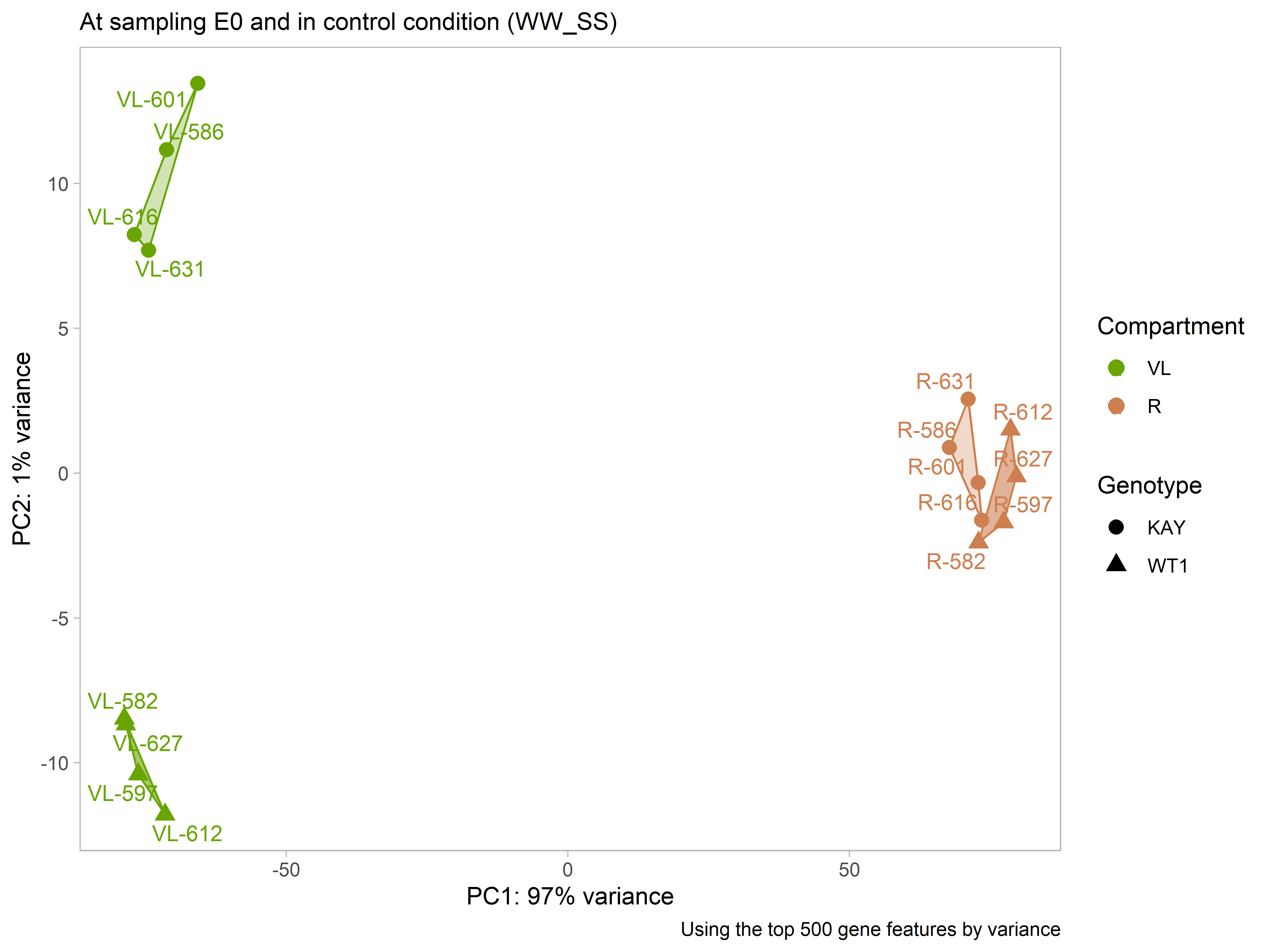 ### List of the gene differentialy express between both genotype for each compartment or both compartment ```{r, eval = F} #parameter lfc_lim_i = 0 pval_i =0.05 resultsNames(dds_comparison_compartment_E0_1) df_vst <- assay(vst_comparison_compartment_E0) Target <- sample_list_rnaseq_comparison_compartment_E0 %>% dplyr::select(genotype, compartment, sample_id) Target=as.data.frame(Target) Target = Target %>% mutate(genotype = as.factor(as.character(genotype)), compartment = as.factor(compartment)) model <- model.matrix(as.formula(paste("~", paste(colnames(Target)[1:2], collapse = " + "), paste(colnames(Target[,1:2]),collapse = ":"), sep = " + ")), data=Target) contrast.matrix = Contrasts(model,Target,FALSE,TRUE) # # mycontrast1 <- c(0, 0, +1, -1, +1, +1, -1, +1) # mycontrast2 <- c(0, 0, +1, -1, +1, 0, 0, 0) contrast.matrix # votre matrice après Contrasts(...) fit <- limma::lmFit(df_vst, model) fit2 <- limma::contrasts.fit(fit, t(contrast.matrix)) fit2 <- limma::eBayes(fit2) p_adj <- apply(fit2$p.value, 2, p.adjust, method = "BH") is_significant <- p_adj < 0.05 # Matrice TRUE/FALSE pour FDR < 0.05 is_upregulated <- is_significant & (fit2$coefficients > lfc_lim_i) # logFC > 0 is_downregulated <- is_significant & (fit2$coefficients < -lfc_lim_i) # logFC < 0 vector_with_interest <- c("[VL-R]", "[KAY-WT1]","[VL_KAY-VL_WT1]", "[R_KAY-R_WT1]", "[KAY_VL-KAY_R]","[WT1_VL-WT1_R]", "[KAY_VL-KAY_R]-[WT1_VL-WT1_R]") summary_DEG <- tibble( Contrast = colnames(fit2$p.value), Upregulated = colSums(is_upregulated), Downregulated = colSums(is_downregulated) ) %>% pivot_longer(cols = -c("Contrast"), names_to = "sign", values_to = "length") %>% mutate(sign = recode(sign, "Upregulated" = "Up", "Downregulated" = "Down")) %>% dplyr::group_by(Contrast) %>% mutate( total = sum(length), percent = round(100 * length / total) ) %>% ungroup() %>% filter(Contrast %in% c(vector_with_interest)) %>% mutate(sign = fct_relevel(sign, c("Up", "Down")), Contrast = fct_relevel(Contrast, rev(vector_with_interest))) # Show results px <- ggplot(summary_DEG, aes(x = Contrast, y = length, fill = sign)) + geom_col() + # 1) Texte pour les barres "assez grandes" (>= 5) geom_text( data = subset(summary_DEG, length >= ifelse(lfc_lim_i == 0, 600,30)), aes( label = paste0(length, "\n(", percent, "%)") ), position = position_stack(vjust = 0.5), color = "white", # texte en blanc size = 3, # hjust = 0.5 (par défaut) - pas indispensable ) + # 2) Texte pour les barres "trop petites" (< 5) geom_text( data = subset(summary_DEG, length < ifelse(lfc_lim_i == 0, 600,30)), aes( label = paste0(length, " (", percent, "%)"), color = sign, # couleur du texte = même code couleur que "sign" vjust = ifelse(sign == "Up", -0.5, 1.5), y=total ), #position = position_stack(vjust = 0.5), hjust= -0.2, # On décale à droite (hors de la barre). En coord_flip(), # hjust < 0 place le texte davantage à droite. #hjust = -0.2, size = 3 ) + theme_minimal() + labs( x = "Comparison", y = "Number of genes deregulated", title = paste0("Number of genes deregulated for each contrast (FDR=0.05 ; LogFC=", lfc_lim_i, ")\nBefor stress") ) + coord_flip() + # Couleurs de remplissage (barres) scale_fill_manual( values = c('Down' = "#1d4877", 'Up' = "#ee3e32"), name = "Sign" ) + # Couleurs du texte (identique aux barres), sans nouvelle légende scale_color_manual( values = c('Down' = "#1d4877", 'Up' = "#ee3e32"), guide = FALSE ) ; px fig_export(path = here::here(paste0("report/rnaseq/plot/genotype_compartment_effect/barplot_differential_expression_lfc_",lfc_lim_i,"_E0_WW_SS")), px, height = 4, width = 10, res_i = 600, format = "png") ################### need to change below ######## # export eatch contrast res_list <- list() # Loop through each contrast in your vector of interest for (contrast in vector_with_interest) { # Construct vector names, e.g., "[SD-SS](Up)" and "[SD-SS](Down)" up_name <- paste0("(Up)", contrast) down_name <- paste0("(Down)", contrast) # Extract the rownames of all Upregulated genes for this contrast genes_up <- rownames(is_upregulated)[is_upregulated[, contrast]] # Extract the rownames of all Downregulated genes for this contrast genes_down <- rownames(is_downregulated)[is_downregulated[, contrast]] # Store them into the result list with meaningful names res_list[[up_name]] <- genes_up res_list[[down_name]] <- genes_down } save(res_list, file = here::here(paste0("data/rnaseq/output/genotype_compartment_effect/contraste_lfc_",lfc_lim_i,"_E0_WW_SS.RData"))) ``` ```{r, eval= F} #parameter lfc_lim_i = 0 pval_i =0.05 load(file = here::here("data/rnaseq/output/comparison_compartment_E0.RData")) load(file = here::here(paste0("data/rnaseq/output/genotype_compartment_effect/contraste_lfc_",lfc_lim_i,"_E0_WW_SS.RData"))) names(res_list) cluster_info <- enframe(res_list, name = "cluster", value = "ID") %>% # -> tibble cluster / liste(ID) unnest(ID) %>% mutate(ID = sub("\\.[0-9]+$", "", ID)) univers_genes<-assay(dds_comparison_compartment_E0) %>% as.data.frame()%>% rownames_to_column("ID") %>% mutate(ID = str_remove(ID, "\\.[0-9]+$")) %>% pull(ID) df_GO = GO_on_different_group(functional_roles = "BP", #"BP" group_info = cluster_info, group = "cluster", ID = "ID", top = 10, universe_i = univers_genes ) # Merge this with your original data to fill missing combinations Cluster_selected_GO_filled <-df_GO %>% # on s'arrete ici pour la fonction. dplyr::rename(cluster = group) %>% mutate(cluster = factor(cluster, levels = unique(cluster)), comparison = str_trim(str_remove(cluster, "\\s*\\(.*?\\)")), sign = str_extract(cluster, "(?<=\\().*?(?=\\))") )# %>% #mutate(comparison = forcats::fct_relevel(comparison, "Mutant vs WT under SS", "Mutant vs WT under SD", "SS_WT vs SD_WT")) #vector_color <- c("#067B5B", "#6AD6AD", "#B87100", "#FFAC5C", "#9381FF", "#067B5B", "#6AD6AD", "#B87100", "#FFAC5C", "#9381FF") # Plot the enrichment by GO px <- ggplot(Cluster_selected_GO_filled, aes(x = cluster, y = Description_GO, fill = `|-log10(Pval)|`)) + geom_tile(color = "black") + scale_fill_gradient2(low = "white", high = "red", na.value = "white", limits = c(0, NA)) + theme_minimal() + theme(axis.text = element_text(size = 8, colour = "black"), axis.text.x = element_text(angle = 90, vjust = 0.5, hjust = 1), panel.grid.major = element_blank(), plot.background = element_rect(fill = "white", colour = "white")) + labs(fill = "-log10(FDR)", x= "Biological process", y = "Cluster", title = "GO terms for all gene deregulated") + #scale_size_manual(values = c(dot = 2, no_dot = NA), guide = "none")+ new_scale_fill() + # scale_fill_manual( # values = c("Mutant vs WT under SS" = as.character(sulfate_pallet[1]), # "Mutant vs WT under SD" = as.character(sulfate_pallet[2]), # "SS_WT vs SD_WT" = "#9381FF"), # name = "Comparison" # ) + scale_fill_brewer(palette = "Dark2", name = "Comparison")+ geom_tile( aes( x = cluster, y = -1, # If you truly want it at a negative y-value, # ensure your y-scale is continuous or can handle this fill = comparison, width = 0.90, height = 0.80 ), data = Cluster_selected_GO_filled, color = "black", alpha = 1, inherit.aes = FALSE )+ new_scale_fill() + scale_fill_manual( values = c('Down' = "#1d4877", 'Up' = "#ee3e32"), name = "Sign" ) + geom_tile( aes( x = cluster, y = -0.05, # If you truly want it at a negative y-value, # ensure your y-scale is continuous or can handle this fill = sign, width = 0.90, height = 0.80 ), data = Cluster_selected_GO_filled, color = "black", alpha = 1, inherit.aes = FALSE ) ; px # export fig_export(path =paste0("report/rnaseq/plot/genotype_compartment_effect/GO/GO_differential_expression_lfc_",lfc_lim_i,"_E0_WW_SS"), plot_x = px, height_i = 12, width_i = 8, res = 600, format = "png") ``` ### Barplot 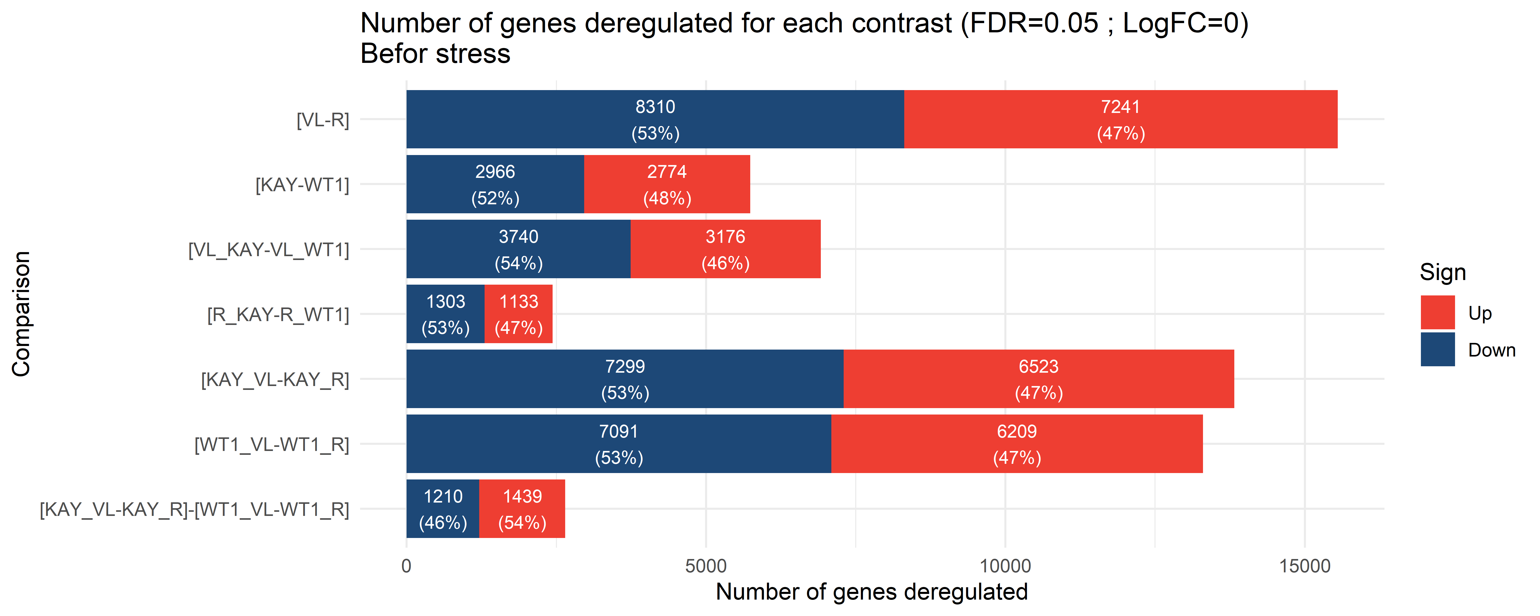 ### GO 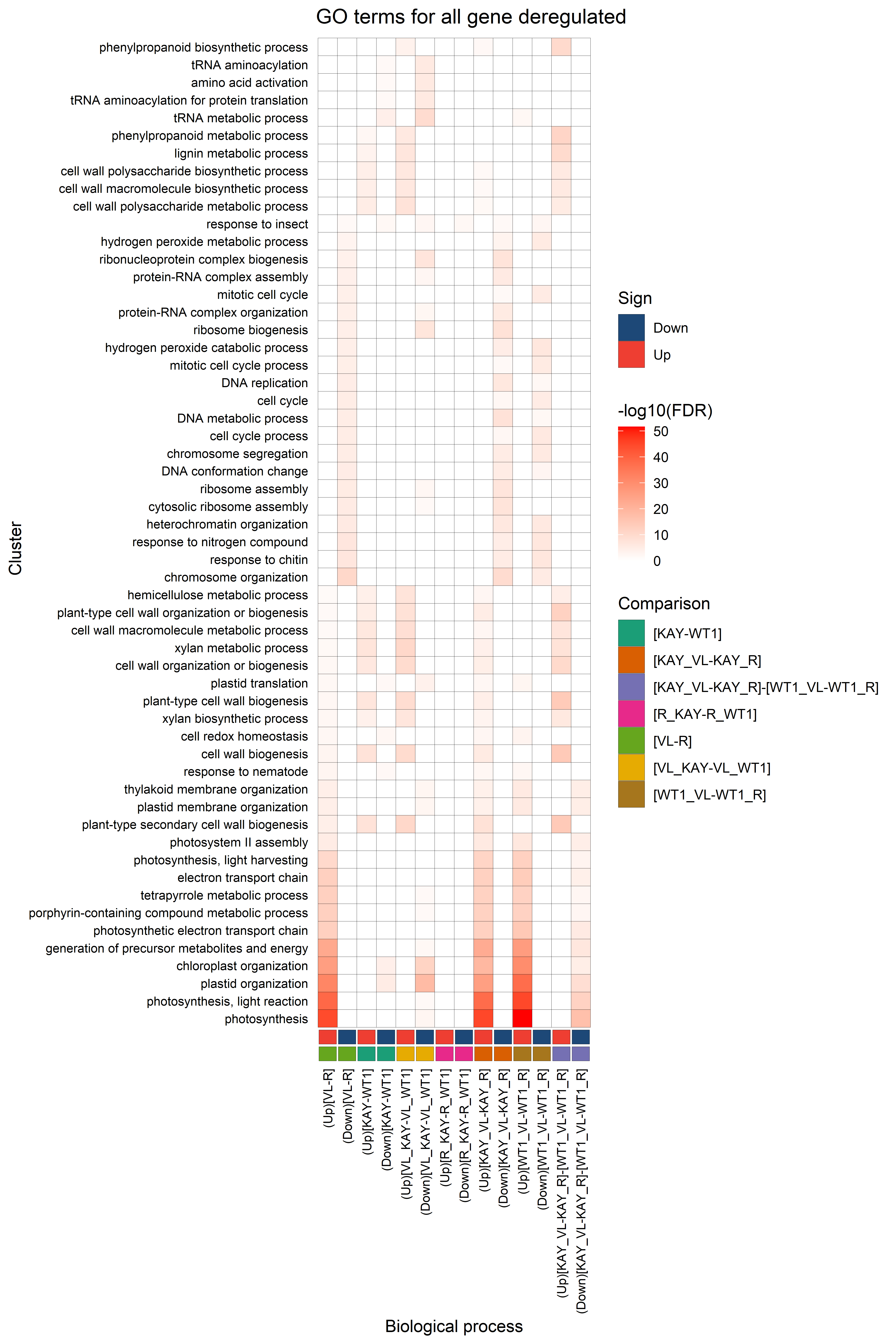 ## For E1 only for control condition and only for WT1 (Cameor) and KAY (Kayane) ### Data importation ```{r} load (file = here:: here ("data/rnaseq/output/comparison_compartment_E1_WW_SS.RData" )) # sample_list_rnaseq_comparison_compartment_E1_WW_SS, dds_comparison_compartment_E1_WW_SS, dds_comparison_compartment_E1_WW_SS_1, rld_comparison_compartment_E1_WW_SS, vst_comparison_compartment_E1_WW_SS ``` ### PCA ```{r, eval = F} # load(file = here::here("data/rnaseq/output/tmp_dds90.RData")) plotMA(dds_comparison_compartment_E1_WW_SS_1) plotDispEsts(dds_comparison_compartment_E1_WW_SS_1) ntop_gene=500 data_PCA<-DESeq2::plotPCA(rld_comparison_compartment_E1_WW_SS, intgroup=c("genotype","compartment"), returnData=TRUE,ntop = ntop_gene) %>% mutate(condition = paste(sep = "_", genotype, compartment)) percentVar <- round(100 * attr(data_PCA, "percentVar")) p1 <- ggplot( data_PCA, aes(PC1, PC2, color = compartment, # <- couleur par compartiment shape = genotype) ) + geom_point(size = 3) + xlab(paste0("PC1: ", percentVar[1], "% variance")) + ylab(paste0("PC2: ", percentVar[2], "% variance")) + theme_light() + theme(panel.grid = element_blank()) + scale_color_manual(values = pallet_compartment)+ scale_fill_manual(values = pallet_compartment)+ geom_text_repel(aes(label = sub(".*\\.", "", name)), size = 3.5) + labs(color = "Compartment", # légende mise à jour shape = "Genotype", subtitle = "At sampling E1 and in control condition (WW_SS)") ## ---- convex-hulls ------------------------------------------------------- hull_data_PCA <- data_PCA |> as_tibble() |> drop_na() |> dplyr::group_by(condition) |> dplyr::slice(chull(PC1, PC2)) |> mutate( alpha_value = ifelse(genotype == "KAY", 0.3, 0.6) # alpha selon génotype ) p2 <- p1 + geom_polygon( data = hull_data_PCA, aes( fill = compartment, # <- même couleur que les points colour = compartment, alpha = alpha_value # transparence conservée ), show.legend = FALSE # on masque la double légende ) + scale_alpha(range = c(0.3, 0.6)) + labs( caption = paste0("Using the top ", ntop_gene, " gene features by variance") ) p2 #export fig_export(here::here(paste0("report/rnaseq/plot/genotype_compartment_effect/PCA_top_",ntop_gene,"_gene_E1_WW_SS")), p2, height_i = 6, width_i = 8, res_i = 600,format = "png") ``` 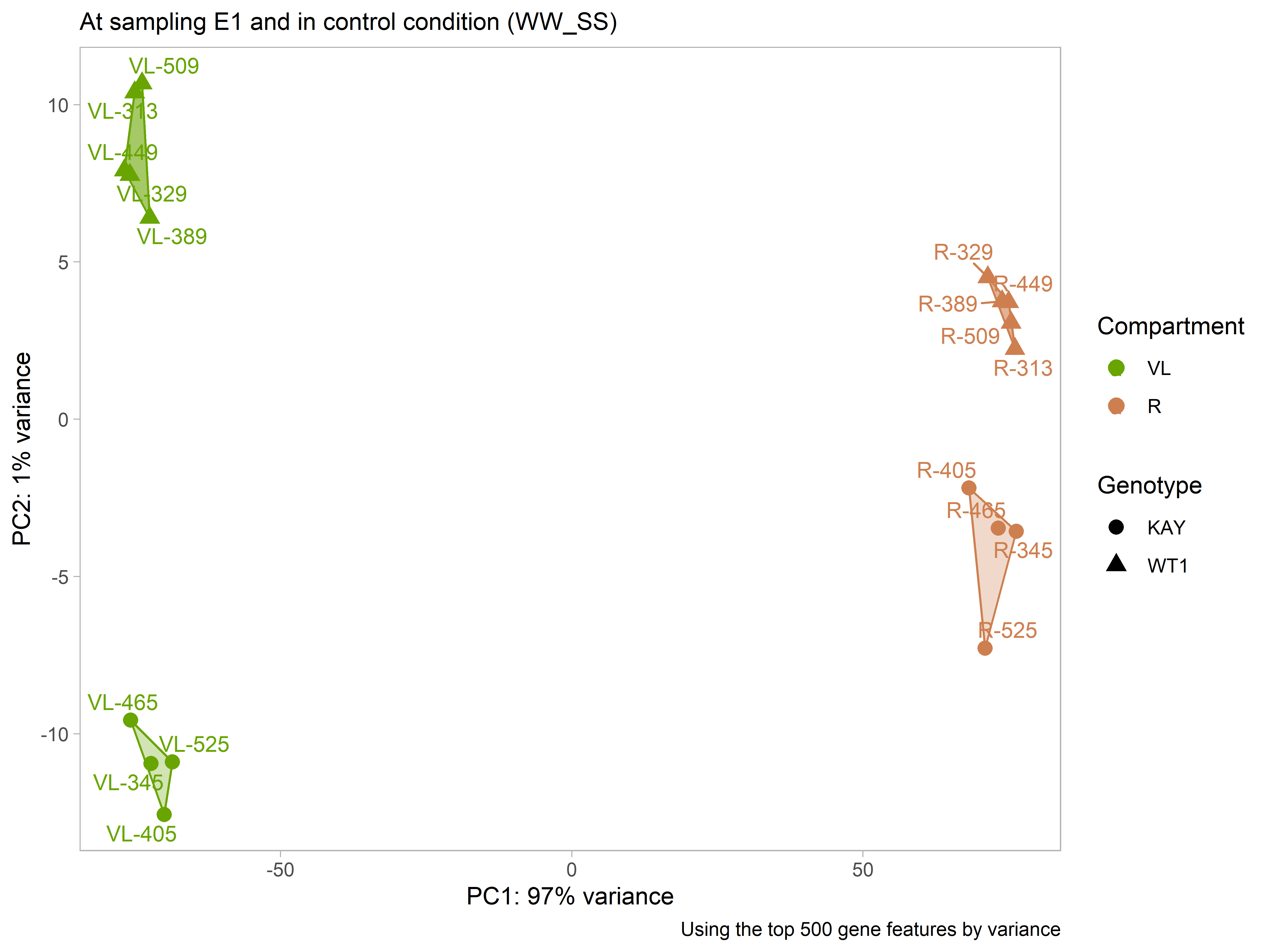 ### List of the gene differentialy express between both genotype for each compartment or both compartment ```{r, eval = F} #parameter lfc_lim_i = 0 pval_i =0.05 resultsNames(dds_comparison_compartment_E1_WW_SS_1) df_vst <- assay(vst_comparison_compartment_E1_WW_SS) Target <- sample_list_rnaseq_comparison_compartment_E1_WW_SS %>% dplyr::select(genotype, compartment, sample_id) Target=as.data.frame(Target) Target = Target %>% mutate(genotype = as.factor(as.character(genotype)), compartment = as.factor(compartment)) model <- model.matrix(as.formula(paste("~", paste(colnames(Target)[1:2], collapse = " + "), paste(colnames(Target[,1:2]),collapse = ":"), sep = " + ")), data=Target) contrast.matrix = Contrasts(model,Target,FALSE,TRUE) # # mycontrast1 <- c(0, 0, +1, -1, +1, +1, -1, +1) # mycontrast2 <- c(0, 0, +1, -1, +1, 0, 0, 0) contrast.matrix # votre matrice après Contrasts(...) fit <- limma::lmFit(df_vst, model) fit2 <- limma::contrasts.fit(fit, t(contrast.matrix)) fit2 <- limma::eBayes(fit2) p_adj <- apply(fit2$p.value, 2, p.adjust, method = "BH") is_significant <- p_adj < 0.05 # Matrice TRUE/FALSE pour FDR < 0.05 is_upregulated <- is_significant & (fit2$coefficients > lfc_lim_i) # logFC > 0 is_downregulated <- is_significant & (fit2$coefficients < -lfc_lim_i) # logFC < 0 vector_with_interest <- c("[VL-R]", "[KAY-WT1]","[VL_KAY-VL_WT1]", "[R_KAY-R_WT1]", "[KAY_VL-KAY_R]","[WT1_VL-WT1_R]", "[KAY_VL-KAY_R]-[WT1_VL-WT1_R]") summary_DEG <- tibble( Contrast = colnames(fit2$p.value), Upregulated = colSums(is_upregulated), Downregulated = colSums(is_downregulated) ) %>% pivot_longer(cols = -c("Contrast"), names_to = "sign", values_to = "length") %>% mutate(sign = recode(sign, "Upregulated" = "Up", "Downregulated" = "Down")) %>% dplyr::group_by(Contrast) %>% mutate( total = sum(length), percent = round(100 * length / total) ) %>% ungroup() %>% filter(Contrast %in% c(vector_with_interest)) %>% mutate(sign = fct_relevel(sign, c("Up", "Down")), Contrast = fct_relevel(Contrast, rev(vector_with_interest))) # Show results px <- ggplot(summary_DEG, aes(x = Contrast, y = length, fill = sign)) + geom_col() + # 1) Texte pour les barres "assez grandes" (>= 5) geom_text( data = subset(summary_DEG, length >= ifelse(lfc_lim_i == 0, 600,30)), aes( label = paste0(length, "\n(", percent, "%)") ), position = position_stack(vjust = 0.5), color = "white", # texte en blanc size = 3, # hjust = 0.5 (par défaut) - pas indispensable ) + # 2) Texte pour les barres "trop petites" (< 5) geom_text( data = subset(summary_DEG, length < ifelse(lfc_lim_i == 0, 600,30)), aes( label = paste0(length, " (", percent, "%)"), color = sign, # couleur du texte = même code couleur que "sign" vjust = ifelse(sign == "Up", -0.5, 1.5), y=total ), #position = position_stack(vjust = 0.5), hjust= -0.2, # On décale à droite (hors de la barre). En coord_flip(), # hjust < 0 place le texte davantage à droite. #hjust = -0.2, size = 3 ) + theme_minimal() + labs( x = "Comparison", y = "Number of genes deregulated", title = paste0("Number of genes deregulated for each contrast (FDR=0.05 ; LogFC=", lfc_lim_i, ")\nAt E1 for control condition (WW_SS)") ) + coord_flip() + # Couleurs de remplissage (barres) scale_fill_manual( values = c('Down' = "#1d4877", 'Up' = "#ee3e32"), name = "Sign" ) + # Couleurs du texte (identique aux barres), sans nouvelle légende scale_color_manual( values = c('Down' = "#1d4877", 'Up' = "#ee3e32"), guide = FALSE ) ; px fig_export(path = here::here(paste0("report/rnaseq/plot/genotype_compartment_effect/barplot_differential_expression_lfc_",lfc_lim_i,"_E1_WW_SS")), px, height = 4, width = 10, res_i = 600, format = "png") ################### need to change below ######## # export eatch contrast res_list <- list() # Loop through each contrast in your vector of interest for (contrast in vector_with_interest) { # Construct vector names, e.g., "[SD-SS](Up)" and "[SD-SS](Down)" up_name <- paste0("(Up)", contrast) down_name <- paste0("(Down)", contrast) # Extract the rownames of all Upregulated genes for this contrast genes_up <- rownames(is_upregulated)[is_upregulated[, contrast]] # Extract the rownames of all Downregulated genes for this contrast genes_down <- rownames(is_downregulated)[is_downregulated[, contrast]] # Store them into the result list with meaningful names res_list[[up_name]] <- genes_up res_list[[down_name]] <- genes_down } save(res_list, file = here::here(paste0("data/rnaseq/output/genotype_compartment_effect/contraste_lfc_",lfc_lim_i,"_E1_WW_SS.RData"))) ``` ```{r, eval= F} #parameter lfc_lim_i = 0 pval_i =0.05 load(file = here::here("data/rnaseq/output/comparison_compartment_E1_WW_SS.RData")) load(file = here::here(paste0("data/rnaseq/output/genotype_compartment_effect/contraste_lfc_",lfc_lim_i,"_E1_WW_SS.RData"))) names(res_list) cluster_info <- enframe(res_list, name = "cluster", value = "ID") %>% # -> tibble cluster / liste(ID) unnest(ID) %>% mutate(ID = sub("\\.[0-9]+$", "", ID)) univers_genes<-assay(dds_comparison_compartment_E1_WW_SS) %>% as.data.frame()%>% rownames_to_column("ID") %>% mutate(ID = str_remove(ID, "\\.[0-9]+$")) %>% pull(ID) df_GO = GO_on_different_group(functional_roles = "BP", #"BP" group_info = cluster_info, group = "cluster", ID = "ID", top = 10, universe_i = univers_genes ) # Merge this with your original data to fill missing combinations Cluster_selected_GO_filled <-df_GO %>% # on s'arrete ici pour la fonction. dplyr::rename(cluster = group) %>% mutate(cluster = factor(cluster, levels = unique(cluster)), comparison = str_trim(str_remove(cluster, "\\s*\\(.*?\\)")), sign = str_extract(cluster, "(?<=\\().*?(?=\\))") )# %>% #mutate(comparison = forcats::fct_relevel(comparison, "Mutant vs WT under SS", "Mutant vs WT under SD", "SS_WT vs SD_WT")) #vector_color <- c("#067B5B", "#6AD6AD", "#B87100", "#FFAC5C", "#9381FF", "#067B5B", "#6AD6AD", "#B87100", "#FFAC5C", "#9381FF") # Plot the enrichment by GO px <- ggplot(Cluster_selected_GO_filled, aes(x = cluster, y = Description_GO, fill = `|-log10(Pval)|`)) + geom_tile(color = "black") + scale_fill_gradient2(low = "white", high = "red", na.value = "white", limits = c(0, NA)) + theme_minimal() + theme(axis.text = element_text(size = 8, colour = "black"), axis.text.x = element_text(angle = 90, vjust = 0.5, hjust = 1), panel.grid.major = element_blank(), plot.background = element_rect(fill = "white", colour = "white")) + labs(fill = "-log10(FDR)", x= "Biological process", y = "Cluster", title = "GO terms for all gene deregulated") + #scale_size_manual(values = c(dot = 2, no_dot = NA), guide = "none")+ new_scale_fill() + # scale_fill_manual( # values = c("Mutant vs WT under SS" = as.character(sulfate_pallet[1]), # "Mutant vs WT under SD" = as.character(sulfate_pallet[2]), # "SS_WT vs SD_WT" = "#9381FF"), # name = "Comparison" # ) + scale_fill_brewer(palette = "Dark2", name = "Comparison")+ geom_tile( aes( x = cluster, y = -1, # If you truly want it at a negative y-value, # ensure your y-scale is continuous or can handle this fill = comparison, width = 0.90, height = 0.80 ), data = Cluster_selected_GO_filled, color = "black", alpha = 1, inherit.aes = FALSE )+ new_scale_fill() + scale_fill_manual( values = c('Down' = "#1d4877", 'Up' = "#ee3e32"), name = "Sign" ) + geom_tile( aes( x = cluster, y = -0.05, # If you truly want it at a negative y-value, # ensure your y-scale is continuous or can handle this fill = sign, width = 0.90, height = 0.80 ), data = Cluster_selected_GO_filled, color = "black", alpha = 1, inherit.aes = FALSE ) ; px # export fig_export(path =paste0("report/rnaseq/plot/genotype_compartment_effect/GO/GO_differential_expression_lfc_",lfc_lim_i,"_E1_WW_SS"), plot_x = px, height_i = 8, width_i = 7.5, res = 600, format = "png") ``` ### Barplot 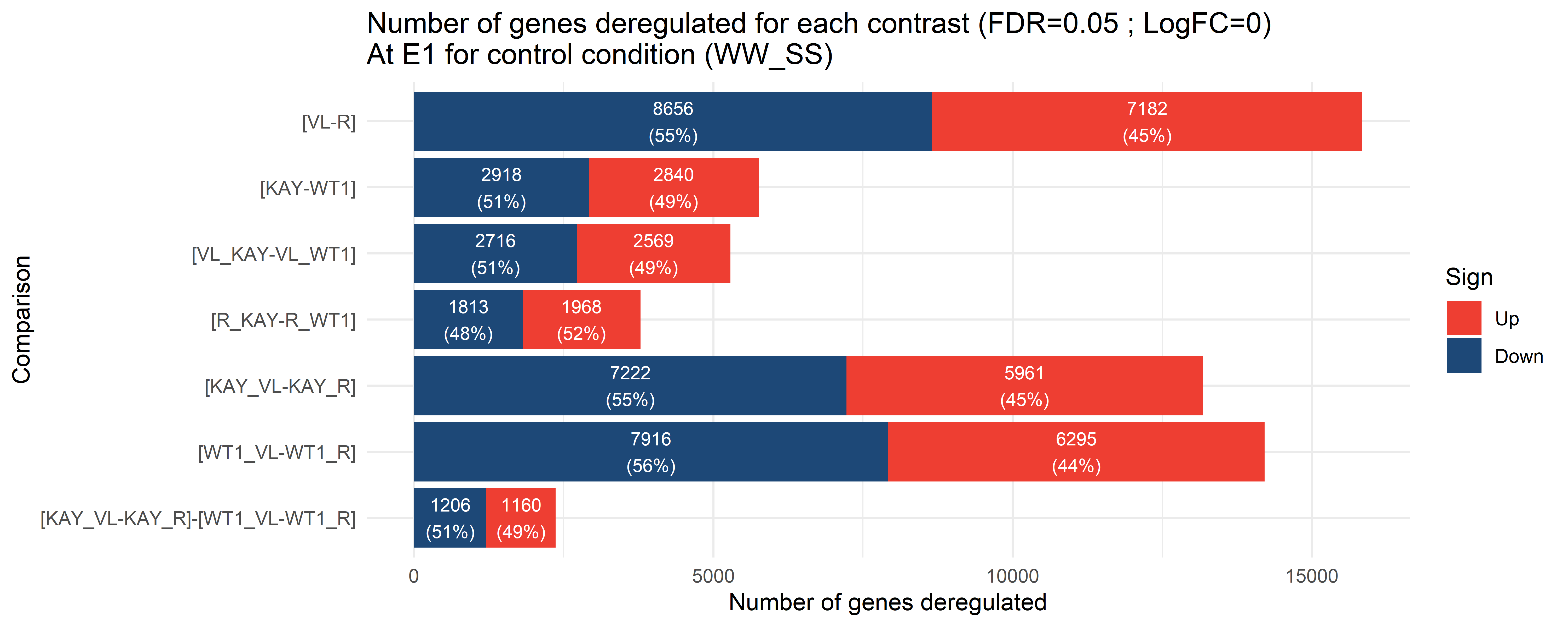 ### GO  ## Both sampling (E0 and E1) in controle condition (WW_SS) ### Data importation ```{r} load (file = here:: here ("data/rnaseq/output/comparison_compartment_E0_E1_WW_SS.RData" )) # sample_list_rnaseq_comparison_compartment_E1_WW_SS, dds_comparison_compartment_E1_WW_SS, dds_comparison_compartment_E1_WW_SS_1, rld_comparison_compartment_E1_WW_SS, vst_comparison_compartment_E1_WW_SS ``` ### PCA ```{r, eval = F} # load(file = here::here("data/rnaseq/output/tmp_dds90.RData")) plotMA(dds_comparison_compartment_E0_E1_WW_SS_1) plotDispEsts(dds_comparison_compartment_E0_E1_WW_SS_1) ntop_gene=1000 data_PCA<-DESeq2::plotPCA(rld_comparison_compartment_E0_E1_WW_SS, intgroup=c("genotype","compartment", "sampling"), returnData=TRUE,ntop = ntop_gene) %>% mutate(condition = paste(sep = "_", genotype, compartment, sampling)) percentVar <- round(100 * attr(data_PCA, "percentVar")) p1 <- ggplot( data_PCA, aes( PC1, PC2, shape = genotype, fill = sampling, colour = compartment ) ) + geom_point(size = 4, stroke = 1.1) + scale_shape_manual(values = c(KAY = 21, WT1 = 22)) + scale_fill_manual( breaks = c("E0", "E1"), values = pallet_sampling, drop = FALSE ) + scale_colour_manual(values = pallet_compartment) + guides( fill = guide_legend(order = 2, override.aes = list(shape = 21)), colour = guide_legend(order = 3, override.aes = list(fill = NA)) ) + xlab(sprintf("PC1 : %s %% de variance", percentVar[1])) + ylab(sprintf("PC2 : %s %% de variance", percentVar[2])) + theme_light() + theme(panel.grid = element_blank()) + geom_text_repel(aes(label = sub(".*\\.", "", name)), size = 3.5) + labs( shape = "Genotype", fill = "Sampling", colour = "Compartment", subtitle = "At sampling E0 and E1 in control condition (WW_SS)" ) + labs( caption = paste0("Using the top ", ntop_gene, " gene features by variance") ); p1 #export fig_export(here::here(paste0("report/rnaseq/plot/genotype_compartment_effect/PCA_top_",ntop_gene,"_gene_E0_E1_WW_SS")), p1, height_i = 6, width_i = 8, res_i = 600,format = "png") ``` 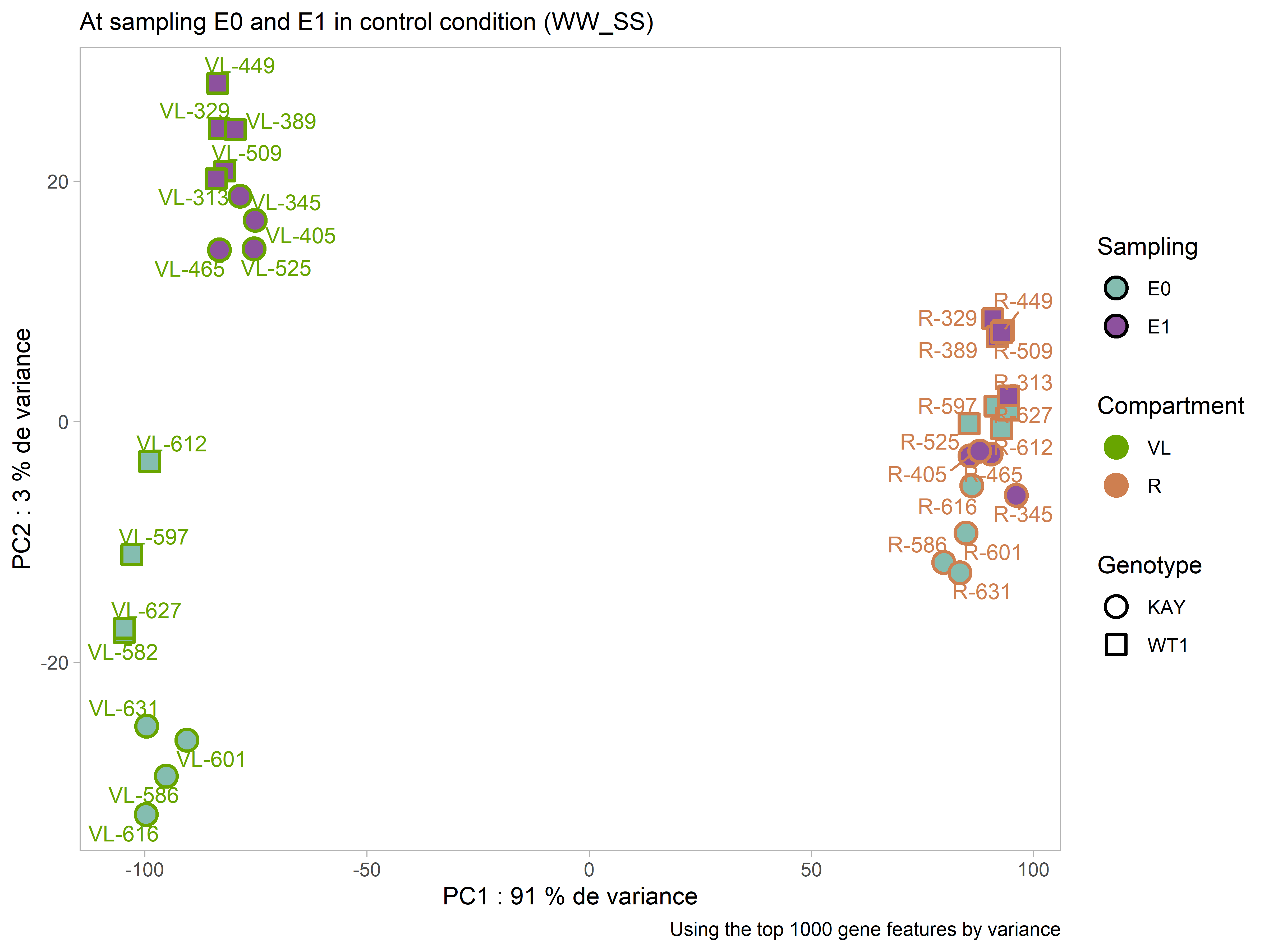 ### List of the gene differentialy express between both genotype for each compartment at E0, E1 ```{r, eval = F} #parameter lfc_lim_i = 0 pval_i =0.05 # Data importation load(file = here::here(paste0("data/rnaseq/output/genotype_compartment_effect/contraste_lfc_",lfc_lim_i,"_E0_WW_SS.RData"))) res_list_E0 = res_list names(res_list_E0) <- paste0(names(res_list_E0), "(E0)") load(file = here::here(paste0("data/rnaseq/output/genotype_compartment_effect/contraste_lfc_",lfc_lim_i,"_E1_WW_SS.RData"))) res_list_E1 = res_list names(res_list_E1) <- paste0(names(res_list_E1), "(E1)") rm(res_list) names(res_list_E0) #euler plot for VL vs R p_VL_R<- list( "(Down)[VL-R](E0)" = res_list_E0[["(Down)[VL-R](E0)"]], "(Down)[VL-R](E1)" = res_list_E1[["(Down)[VL-R](E1)"]], "(Up)[VL-R](E0)" = res_list_E0[["(Up)[VL-R](E0)"]], "(Up)[VL-R](E1)" = res_list_E1[["(Up)[VL-R](E1)"]] ) euler_VL_R <- plot(eulerr::euler(p_VL_R, shape = "ellipse"), quantities = TRUE, fills = c(lighten("#1d4877", amount = -.1), lighten(as.character("#1d4877"), amount = .6), lighten("#ee3e32", amount = -.1), lighten("#ee3e32", amount = .6)), legend = list(side = "right"), main = list(label = "Euler diagram of down and up regulated genes for difference between R and L", cex = 1.3)) p_KAY_WT1<- list( "(Down)[KAY-WT1](E0)" = res_list_E0[["(Down)[KAY-WT1](E0)"]], "(Down)[KAY-WT1](E1)" = res_list_E1[["(Down)[KAY-WT1](E1)"]], "(Up)[KAY-WT1](E0)" = res_list_E0[["(Up)[KAY-WT1](E0)"]], "(Up)[KAY-WT1](E1)" = res_list_E1[["(Up)[KAY-WT1](E1)"]] ) euler_KAY_WT1 <- plot(eulerr::euler(p_KAY_WT1, shape = "ellipse"), quantities = TRUE, fills = c(lighten("#1d4877", amount = -.1), lighten(as.character("#1d4877"), amount = .6), lighten("#ee3e32", amount = -.1), lighten("#ee3e32", amount = .6)), legend = list(side = "right"), main = list(label = "Euler diagram of down and up regulated genes for difference between KAY and WT1 dosent mater the compartment", cex = 1.3)) p_VL_KAY_VL_WT1<- list( "(Down)[VL_KAY-VL_WT1](E0)" = res_list_E0[["(Down)[VL_KAY-VL_WT1](E0)"]], "(Down)[VL_KAY-VL_WT1](E1)" = res_list_E1[["(Down)[VL_KAY-VL_WT1](E1)"]], "(Up)[VL_KAY-VL_WT1](E0)" = res_list_E0[["(Up)[VL_KAY-VL_WT1](E0)"]], "(Up)[VL_KAY-VL_WT1](E1)" = res_list_E1[["(Up)[VL_KAY-VL_WT1](E1)"]] ) euler_VL_KAY_VL_WT1 <- plot(eulerr::euler(p_VL_KAY_VL_WT1, shape = "ellipse"), quantities = TRUE, fills = c(lighten("#1d4877", amount = -.1), lighten(as.character("#1d4877"), amount = .6), lighten("#ee3e32", amount = -.1), lighten("#ee3e32", amount = .6)), legend = list(side = "right"), main = list(label = "\nEuler diagram of down and up regulated genes for \ndifference between KAY and WT1 only for vegetative leaf", cex = 1.3)) p_R_KAY_R_WT1<- list( "(Down)[R_KAY-R_WT1](E0)" = res_list_E0[["(Down)[R_KAY-R_WT1](E0)"]], "(Down)[R_KAY-R_WT1](E1)" = res_list_E1[["(Down)[R_KAY-R_WT1](E1)"]], "(Up)[R_KAY-R_WT1](E0)" = res_list_E0[["(Up)[R_KAY-R_WT1](E0)"]], "(Up)[R_KAY-R_WT1](E1)" = res_list_E1[["(Up)[R_KAY-R_WT1](E1)"]] ) euler_R_KAY_R_WT1 <- plot(eulerr::euler(p_R_KAY_R_WT1, shape = "ellipse"), quantities = TRUE, fills = c(lighten("#1d4877", amount = -.1), lighten(as.character("#1d4877"), amount = .6), lighten("#ee3e32", amount = -.1), lighten("#ee3e32", amount = .6)), legend = list(side = "right"), main = list(label = "Euler diagram of down and up regulated genes for \ndifference between KAY and WT1 only for root", cex = 1.3)) fig_export(path = here::here(paste0("report/rnaseq/plot/genotype_compartment_effect/euler_VL_lfc_",lfc_lim_i)), euler_VL_KAY_VL_WT1, height = 6, width = 8, res_i = 600, format = "png") fig_export(path = here::here(paste0("report/rnaseq/plot/genotype_compartment_effect/euler_R_lfc_",lfc_lim_i)), euler_R_KAY_R_WT1, height = 6, width = 8, res_i = 600, format = "png") ``` 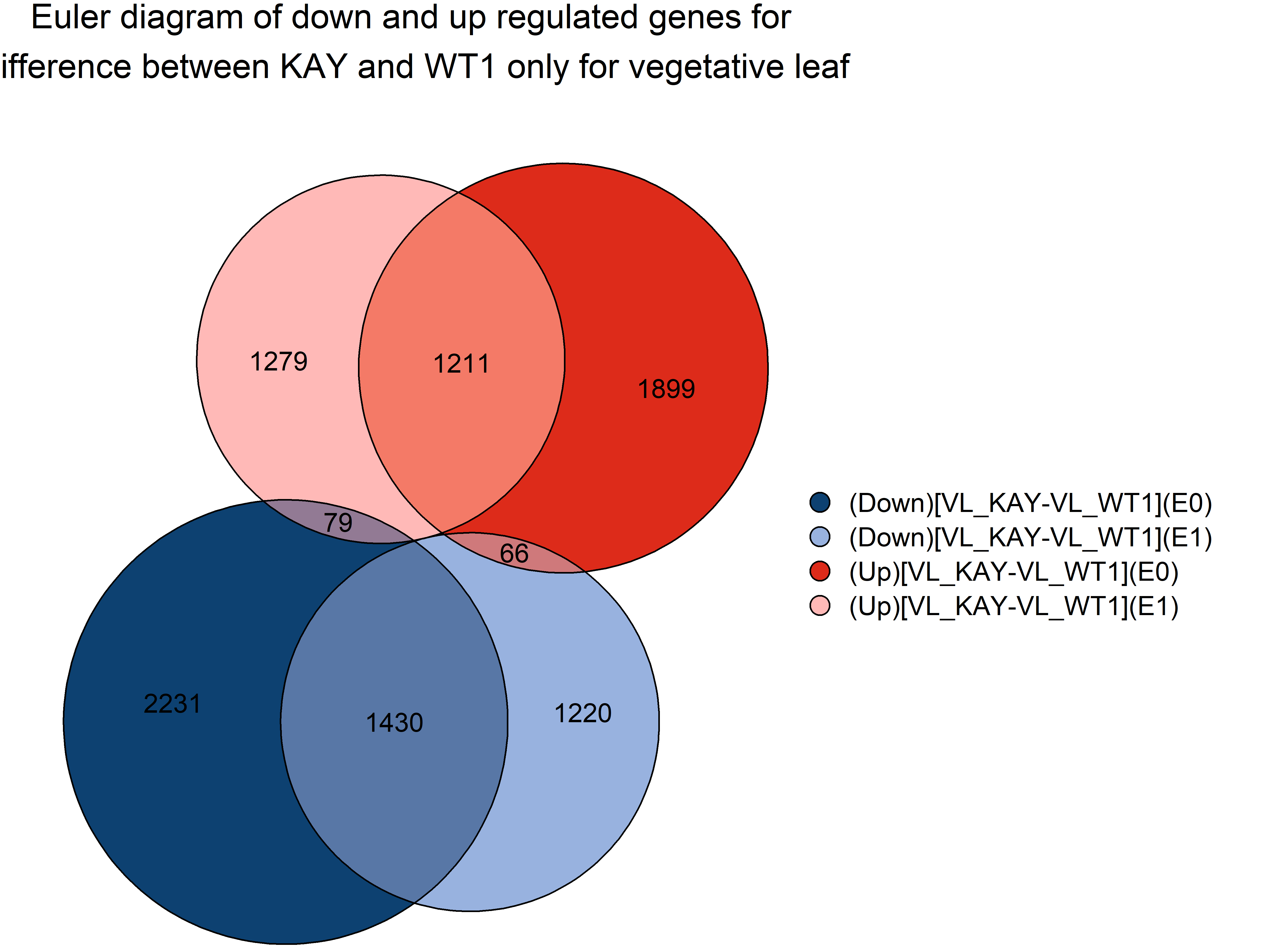 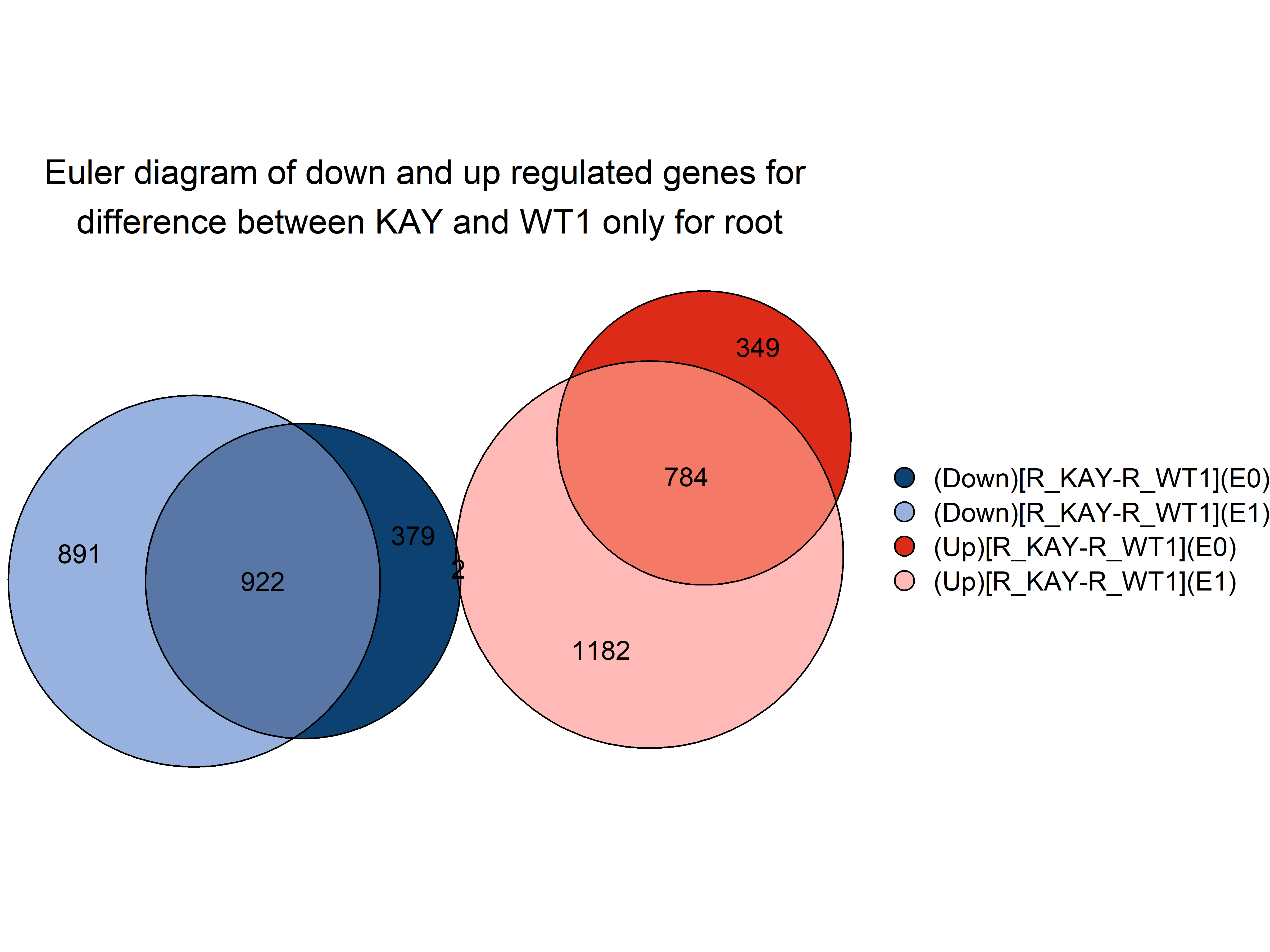 ## If i separate VL and R before DESeq2 to have E2 for Root ### Data importation ```{r} # For leaf load (file = here:: here ("data/rnaseq/output/comparison_genotype_E0_E1_WW_SS_VL.RData" )) # sample_list_rnaseq_comparison_genotype_E0_E1_WW_SS_VL, dds_comparison_genotype_E0_E1_WW_SS_VL, dds_comparison_genotype_E0_E1_WW_SS_VL_1, rld_comparison_genotype_E0_E1_WW_SS_VL, vst_comparison_genotype_E0_E1_WW_SS_VL # For root load (file = here:: here ("data/rnaseq/output/comparison_compartment_E0_E1_E2_WW_SS_R.RData" )) # sample_list_rnaseq_comparison_compartment_E0_E1_E2_WW_SS_R, dds_comparison_compartment_E0_E1_E2_WW_SS_R, dds_comparison_compartment_E0_E1_E2_WW_SS_R_1, rld_comparison_compartment_E0_E1_E2_WW_SS_R, vst_comparison_compartment_E0_E1_E2_WW_SS_R ``` ### PCA ```{r, eval = F} ###################### for LEAF ################## # load(file = here::here("data/rnaseq/output/tmp_dds90.RData")) plotMA(dds_comparison_genotype_E0_E1_WW_SS_VL_1) plotDispEsts(dds_comparison_genotype_E0_E1_WW_SS_VL_1) ntop_gene=1000 data_PCA<-DESeq2::plotPCA(rld_comparison_genotype_E0_E1_WW_SS_VL, intgroup=c("genotype","sampling"), returnData=TRUE,ntop = ntop_gene) %>% mutate(condition = paste(sep = "_", genotype, sampling)) percentVar <- round(100 * attr(data_PCA, "percentVar")) p1 <- ggplot( data_PCA, aes(PC1, PC2, color = sampling, # <- couleur par compartiment shape = genotype) ) + geom_point(size = 3) + xlab(paste0("PC1: ", percentVar[1], "% variance")) + ylab(paste0("PC2: ", percentVar[2], "% variance")) + theme_light() + theme(panel.grid = element_blank()) + scale_color_manual(values = pallet_sampling)+ scale_fill_manual(values = pallet_sampling)+ geom_text_repel(aes(label = sub(".*\\.", "", name)), size = 3.5) + labs(color = "Sampling", # légende mise à jour shape = "Genotype", subtitle = "At sampling E1 and E2 in control condition (WW_SS) only for VL", caption = paste0("Using the top ", ntop_gene, " gene features by variance")) ## ---- convex-hulls ------------------------------------------------------- hull_data_PCA <- data_PCA |> as_tibble() |> drop_na() |> dplyr::group_by(condition) |> dplyr::slice(chull(PC1, PC2)) |> mutate( alpha_value = ifelse(genotype == "KAY", 0.3, 0.6) # alpha selon génotype ) p2_VL <- p1 + geom_polygon( data = hull_data_PCA, aes( fill = sampling, # <- même couleur que les points colour = sampling, alpha = alpha_value # transparence conservée ), show.legend = FALSE # on masque la double légende ) + scale_alpha(range = c(0.3, 0.6)) p2_VL #export fig_export(here::here(paste0("report/rnaseq/plot/genotype_compartment_effect/PCA_top_",ntop_gene,"_gene_E0_E1_WW_SS_VL")), p2_VL, height_i = 6, width_i = 8, res_i = 600,format = "png") ###################### for ROOT ################## # load(file = here::here("data/rnaseq/output/tmp_dds90.RData")) plotMA(dds_comparison_compartment_E0_E1_E2_WW_SS_R_1) plotDispEsts(dds_comparison_compartment_E0_E1_E2_WW_SS_R_1) ntop_gene=1000 data_PCA<-DESeq2::plotPCA(rld_comparison_compartment_E0_E1_E2_WW_SS_R, intgroup=c("genotype","sampling"), returnData=TRUE,ntop = ntop_gene) %>% mutate(condition = paste(sep = "_", genotype, sampling)) percentVar <- round(100 * attr(data_PCA, "percentVar")) p1 <- ggplot( data_PCA, aes(PC1, PC2, color = sampling, # <- couleur par compartiment shape = genotype) ) + geom_point(size = 3) + xlab(paste0("PC1: ", percentVar[1], "% variance")) + ylab(paste0("PC2: ", percentVar[2], "% variance")) + theme_light() + theme(panel.grid = element_blank()) + scale_color_manual(values = pallet_sampling)+ scale_fill_manual(values = pallet_sampling)+ geom_text_repel(aes(label = sub(".*\\.", "", name)), size = 3.5) + labs(color = "Sampling", # légende mise à jour shape = "Genotype", subtitle = "At sampling E1 and E2 in control condition (WW_SS) only for R", caption = paste0("Using the top ", ntop_gene, " gene features by variance")) ## ---- convex-hulls ------------------------------------------------------- hull_data_PCA <- data_PCA |> as_tibble() |> drop_na() |> dplyr::group_by(condition) |> dplyr::slice(chull(PC1, PC2)) |> mutate( alpha_value = ifelse(genotype == "KAY", 0.3, 0.6) # alpha selon génotype ) p2_R <- p1 + geom_polygon( data = hull_data_PCA, aes( fill = sampling, # <- même couleur que les points colour = sampling, alpha = alpha_value # transparence conservée ), show.legend = FALSE # on masque la double légende ) + scale_alpha(range = c(0.3, 0.6)) p2_R p2_VL_no_legende <- p2_VL + theme(legend.position = "none") # combine compartment combined <- (p2_VL_no_legende | p2_R) + # | = côte à côte plot_layout(guides = "collect") & # ne collectera PLUS que la légende de p2 theme(legend.position = "bottom") # place la légende globale où tu veux combined #export fig_export(here::here(paste0("report/rnaseq/plot/genotype_compartment_effect/PCA_top_",ntop_gene,"_gene_E0_E1_E2_WW_SS_R")), p2_R, height_i = 6, width_i = 8, res_i = 600,format = "png") fig_export(here::here(paste0("report/rnaseq/plot/genotype_compartment_effect/PCA_top_",ntop_gene,"_gene_E0_E1_E2_WW_SS_VL_and_R")), combined, height_i = 6, width_i = 14, res_i = 600,format = "png") ``` 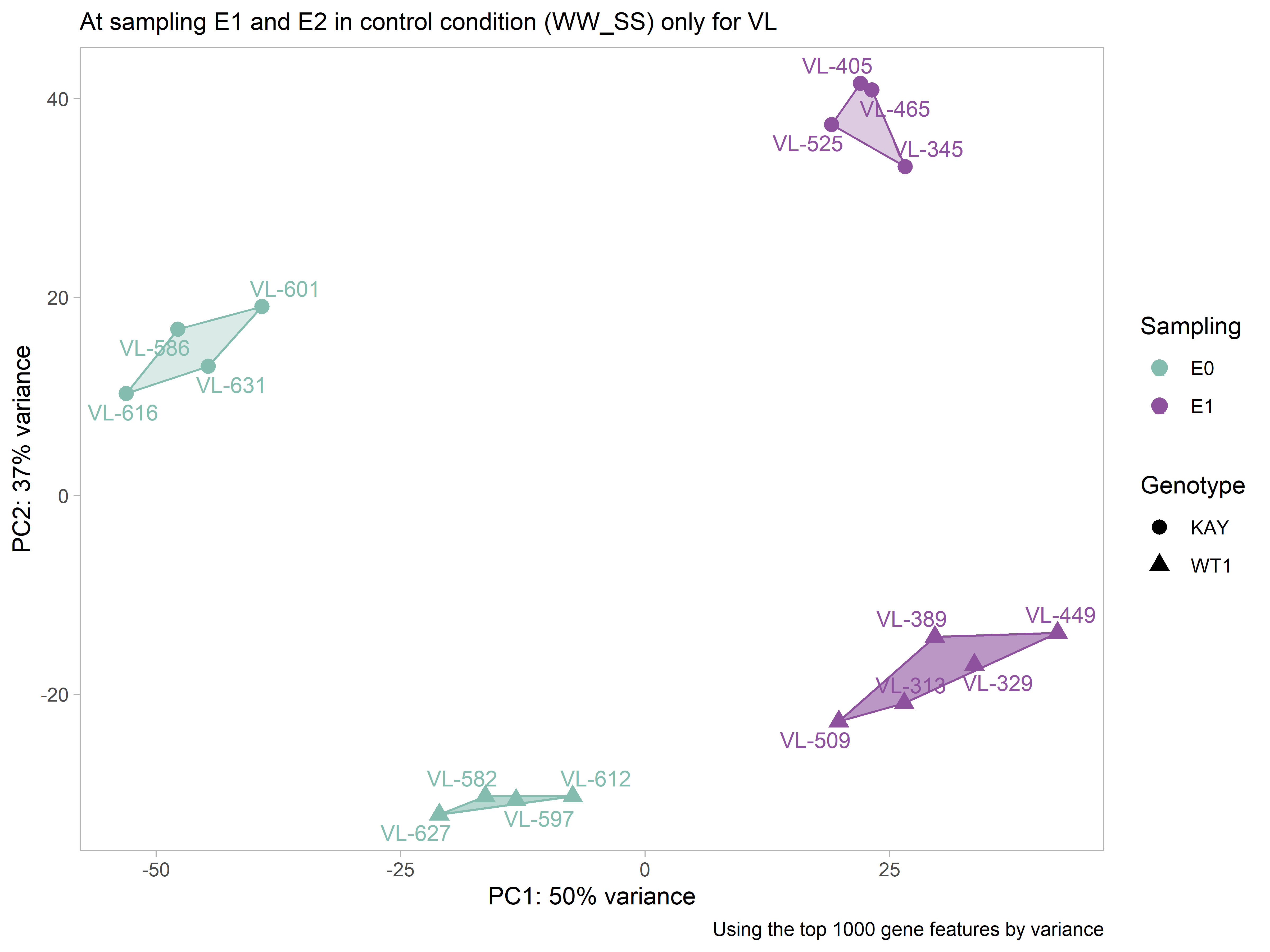 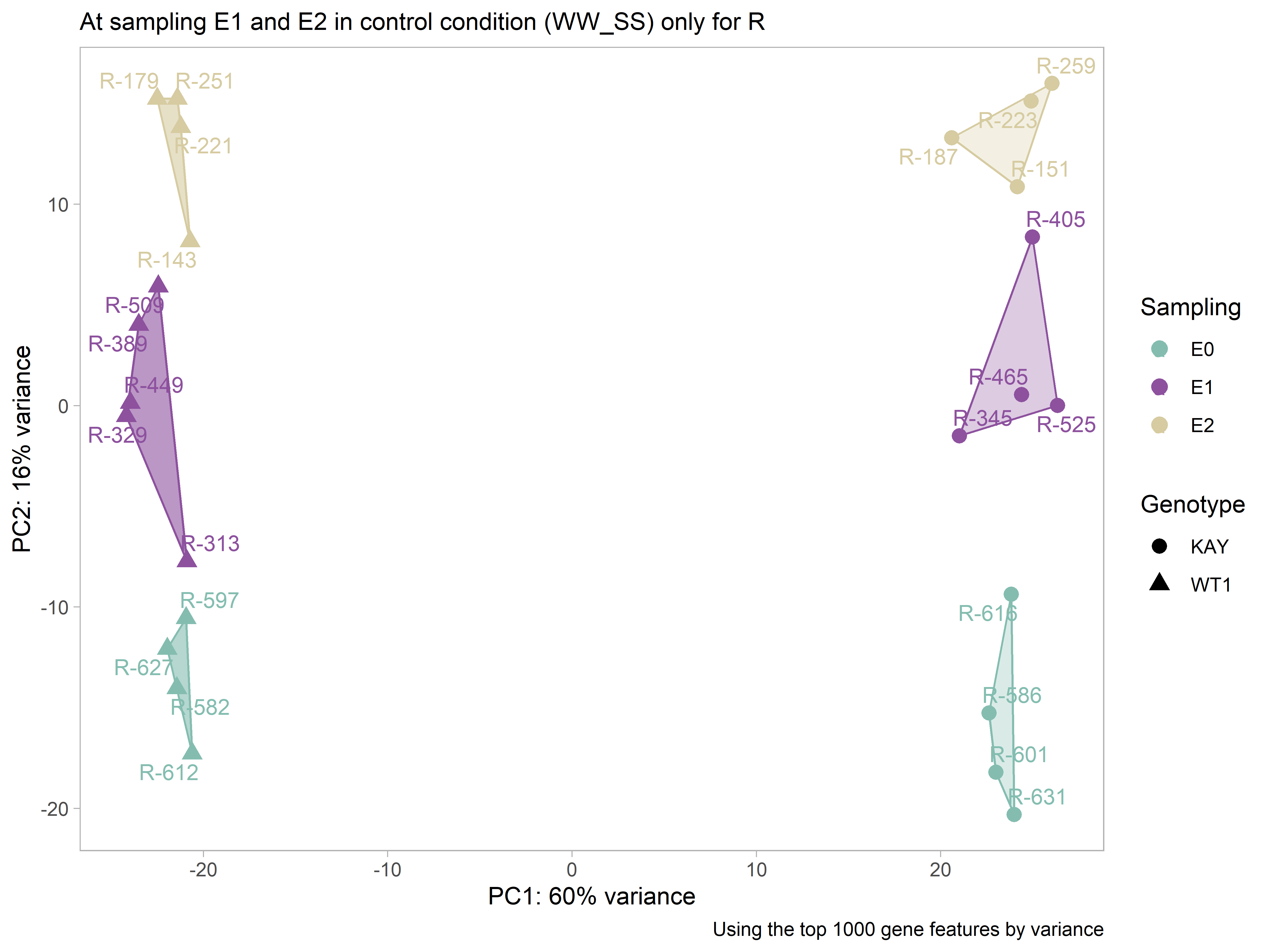 ### List of the gene differentialy express between both genotype for each compartment at E0; E1 and E2 ```{r, eval = F} #parameter lfc_lim_i = 0 pval_i =0.05 ################## VL #################################### resultsNames(dds_comparison_genotype_E0_E1_WW_SS_VL_1) df_vst <- assay(vst_comparison_genotype_E0_E1_WW_SS_VL) Target <- sample_list_rnaseq_comparison_genotype_E0_E1_WW_SS_VL %>% dplyr::select(genotype,sampling, sample_id) Target=as.data.frame(Target) Target = Target %>% mutate(genotype = as.factor(as.character(genotype)), sampling = as.factor(as.character(sampling))) model <- model.matrix(as.formula(paste("~", paste(colnames(Target)[1:2], collapse = " + "), paste(colnames(Target[,1:2]),collapse = ":"), sep = " + ")), data=Target) contrast.matrix = Contrasts(model,Target,FALSE,TRUE) # # mycontrast1 <- c(0, 0, +1, -1, +1, +1, -1, +1) # mycontrast2 <- c(0, 0, +1, -1, +1, 0, 0, 0) contrast.matrix # votre matrice après Contrasts(...) fit <- limma::lmFit(df_vst, model) fit2 <- limma::contrasts.fit(fit, t(contrast.matrix)) fit2 <- limma::eBayes(fit2) p_adj <- apply(fit2$p.value, 2, p.adjust, method = "BH") is_significant <- p_adj < 0.05 # Matrice TRUE/FALSE pour FDR < 0.05 is_upregulated <- is_significant & (fit2$coefficients > lfc_lim_i) # logFC > 0 is_downregulated <- is_significant & (fit2$coefficients < -lfc_lim_i) # logFC < 0 vector_with_interest <- c("[KAY-WT1]", "[E0-E1]","[E0_KAY-E0_WT1]", "[E1_KAY-E1_WT1]", "[KAY_E0-KAY_E1]","[WT1_E0-WT1_E1]", "[KAY_E0-KAY_E1]-[WT1_E0-WT1_E1]") summary_DEG <- tibble( Contrast = colnames(fit2$p.value), Upregulated = colSums(is_upregulated), Downregulated = colSums(is_downregulated) ) %>% pivot_longer(cols = -c("Contrast"), names_to = "sign", values_to = "length") %>% mutate(sign = recode(sign, "Upregulated" = "Up", "Downregulated" = "Down")) %>% dplyr::group_by(Contrast) %>% mutate( total = sum(length), percent = round(100 * length / total) ) %>% ungroup() %>% filter(Contrast %in% c(vector_with_interest)) %>% mutate(sign = fct_relevel(sign, c("Up", "Down")), Contrast = fct_relevel(Contrast, rev(vector_with_interest))) # Show results px <- ggplot(summary_DEG, aes(x = Contrast, y = length, fill = sign)) + geom_col() + # 1) Texte pour les barres "assez grandes" (>= 5) geom_text( data = subset(summary_DEG, length >= ifelse(lfc_lim_i == 0, 600,30)), aes( label = paste0(length, "\n(", percent, "%)") ), position = position_stack(vjust = 0.5), color = "white", # texte en blanc size = 3, # hjust = 0.5 (par défaut) - pas indispensable ) + # 2) Texte pour les barres "trop petites" (< 5) geom_text( data = subset(summary_DEG, length < ifelse(lfc_lim_i == 0, 600,30)), aes( label = paste0(length, " (", percent, "%)"), color = sign, # couleur du texte = même code couleur que "sign" vjust = ifelse(sign == "Up", -0.5, 1.5), y=total ), #position = position_stack(vjust = 0.5), hjust= -0.2, # On décale à droite (hors de la barre). En coord_flip(), # hjust < 0 place le texte davantage à droite. #hjust = -0.2, size = 3 ) + theme_minimal() + labs( x = "Comparison", y = "Number of genes deregulated", title = paste0("Number of genes deregulated for each contrast (FDR=0.05 ; LogFC=", lfc_lim_i, ")\nAt E0 and E1 for control condition (WW_SS) in vegetative leaves") ) + coord_flip() + # Couleurs de remplissage (barres) scale_fill_manual( values = c('Down' = "#1d4877", 'Up' = "#ee3e32"), name = "Sign" ) + # Couleurs du texte (identique aux barres), sans nouvelle légende scale_color_manual( values = c('Down' = "#1d4877", 'Up' = "#ee3e32"), guide = FALSE ) ; px fig_export(path = here::here(paste0("report/rnaseq/plot/genotype_compartment_effect/barplot_differential_expression_lfc_",lfc_lim_i,"_E0_E1_WW_SS_VL")), px, height = 4, width = 10, res_i = 600, format = "png") ################### need to change below ######## # export eatch contrast res_list <- list() # Loop through each contrast in your vector of interest for (contrast in vector_with_interest) { # Construct vector names, e.g., "[SD-SS](Up)" and "[SD-SS](Down)" up_name <- paste0("(Up)", contrast) down_name <- paste0("(Down)", contrast) # Extract the rownames of all Upregulated genes for this contrast genes_up <- rownames(is_upregulated)[is_upregulated[, contrast]] # Extract the rownames of all Downregulated genes for this contrast genes_down <- rownames(is_downregulated)[is_downregulated[, contrast]] # Store them into the result list with meaningful names res_list[[up_name]] <- genes_up res_list[[down_name]] <- genes_down } save(res_list, file = here::here(paste0("data/rnaseq/output/genotype_compartment_effect/contraste_lfc_",lfc_lim_i,"_E0_E1_WW_SS_VL.RData"))) ################## For Root #################################### resultsNames(dds_comparison_compartment_E0_E1_E2_WW_SS_R_1) df_vst <- assay(vst_comparison_compartment_E0_E1_E2_WW_SS_R) Target <- sample_list_rnaseq_comparison_compartment_E0_E1_E2_WW_SS_R %>% dplyr::select(genotype,sampling, sample_id) Target=as.data.frame(Target) Target = Target %>% mutate(genotype = as.factor(as.character(genotype)), sampling = as.factor(sampling)) model <- model.matrix(as.formula(paste("~", paste(colnames(Target)[1:2], collapse = " + "), paste(colnames(Target[,1:2]),collapse = ":"), sep = " + ")), data=Target) contrast.matrix = Contrasts(model,Target,FALSE,TRUE) # # mycontrast1 <- c(0, 0, +1, -1, +1, +1, -1, +1) # mycontrast2 <- c(0, 0, +1, -1, +1, 0, 0, 0) contrast.matrix # votre matrice après Contrasts(...) fit <- limma::lmFit(df_vst, model) fit2 <- limma::contrasts.fit(fit, t(contrast.matrix)) fit2 <- limma::eBayes(fit2) p_adj <- apply(fit2$p.value, 2, p.adjust, method = "BH") is_significant <- p_adj < 0.05 # Matrice TRUE/FALSE pour FDR < 0.05 is_upregulated <- is_significant & (fit2$coefficients > lfc_lim_i) # logFC > 0 is_downregulated <- is_significant & (fit2$coefficients < -lfc_lim_i) # logFC < 0 vector_with_interest <- c("[KAY-WT1]", "[E0-E1]","[E0-E2]","[E1-E2]","[E0_KAY-E0_WT1]", "[E1_KAY-E1_WT1]", "[E2_KAY-E2_WT1]", "[KAY_E0-KAY_E1]", "[KAY_E0-KAY_E2]", "[KAY_E1-KAY_E2]", "[WT1_E0-WT1_E1]", "[WT1_E0-WT1_E2]", "[WT1_E1-WT1_E2]", "[KAY_E0-KAY_E1]-[WT1_E0-WT1_E1]", "[KAY_E0-KAY_E2]-[WT1_E0-WT1_E2]", "[KAY_E1-KAY_E2]-[WT1_E1-WT1_E2]") summary_DEG <- tibble( Contrast = colnames(fit2$p.value), Upregulated = colSums(is_upregulated), Downregulated = colSums(is_downregulated) ) %>% pivot_longer(cols = -c("Contrast"), names_to = "sign", values_to = "length") %>% mutate(sign = recode(sign, "Upregulated" = "Up", "Downregulated" = "Down")) %>% dplyr::group_by(Contrast) %>% mutate( total = sum(length), percent = round(100 * length / total) ) %>% ungroup() %>% filter(Contrast %in% c(vector_with_interest)) %>% mutate(sign = fct_relevel(sign, c("Up", "Down")), Contrast = fct_relevel(Contrast, rev(vector_with_interest))) # Show results px <- ggplot(summary_DEG, aes(x = Contrast, y = length, fill = sign)) + geom_col() + # 1) Texte pour les barres "assez grandes" (>= 5) geom_text( data = subset(summary_DEG, length >= ifelse(lfc_lim_i == 0, 600,30)), aes( label = paste0(length, "\n(", percent, "%)") ), position = position_stack(vjust = 0.5), color = "white", # texte en blanc size = 3, # hjust = 0.5 (par défaut) - pas indispensable ) + # 2) Texte pour les barres "trop petites" (< 5) geom_text( data = subset(summary_DEG, length < ifelse(lfc_lim_i == 0, 600,30)), aes( label = paste0(length, " (", percent, "%)"), color = sign, # couleur du texte = même code couleur que "sign" vjust = ifelse(sign == "Up", -0.5, 1.5), y=total ), #position = position_stack(vjust = 0.5), hjust= -0.2, # On décale à droite (hors de la barre). En coord_flip(), # hjust < 0 place le texte davantage à droite. #hjust = -0.2, size = 3 ) + theme_minimal() + labs( x = "Comparison", y = "Number of genes deregulated", title = paste0("Number of genes deregulated for each contrast (FDR=0.05 ; LogFC=", lfc_lim_i, ")\nAt E0, E1 and E2 for control condition (WW_SS) in roots") ) + coord_flip() + # Couleurs de remplissage (barres) scale_fill_manual( values = c('Down' = "#1d4877", 'Up' = "#ee3e32"), name = "Sign" ) + # Couleurs du texte (identique aux barres), sans nouvelle légende scale_color_manual( values = c('Down' = "#1d4877", 'Up' = "#ee3e32"), guide = FALSE ) ; px fig_export(path = here::here(paste0("report/rnaseq/plot/genotype_compartment_effect/barplot_differential_expression_lfc_",lfc_lim_i,"_E0_E1_E2_WW_SS_R")), px, height = 8, width = 10, res_i = 600, format = "png") ################### need to change below ######## # export eatch contrast res_list <- list() # Loop through each contrast in your vector of interest for (contrast in vector_with_interest) { # Construct vector names, e.g., "[SD-SS](Up)" and "[SD-SS](Down)" up_name <- paste0("(Up)", contrast) down_name <- paste0("(Down)", contrast) # Extract the rownames of all Upregulated genes for this contrast genes_up <- rownames(is_upregulated)[is_upregulated[, contrast]] # Extract the rownames of all Downregulated genes for this contrast genes_down <- rownames(is_downregulated)[is_downregulated[, contrast]] # Store them into the result list with meaningful names res_list[[up_name]] <- genes_up res_list[[down_name]] <- genes_down } save(res_list, file = here::here(paste0("data/rnaseq/output/genotype_compartment_effect/contraste_lfc_",lfc_lim_i,"_E0_E1_E2_WW_SS_R.RData"))) ``` ```{r, eval= F} #parameter lfc_lim_i = 0 pval_i =0.05 ############ for leaf load(file = here::here("data/rnaseq/output/comparison_genotype_E0_E1_WW_SS_VL.RData")) # sample_list_rnaseq_comparison_genotype_E0_E1_WW_SS_VL, dds_comparison_genotype_E0_E1_WW_SS_VL, dds_comparison_genotype_E0_E1_WW_SS_VL_1, rld_comparison_genotype_E0_E1_WW_SS_VL, vst_comparison_genotype_E0_E1_WW_SS_VL load(file = here::here(paste0("data/rnaseq/output/genotype_compartment_effect/contraste_lfc_",lfc_lim_i,"_E0_E1_WW_SS_VL.RData"))) names(res_list) univers_genes<-assay(dds_comparison_genotype_E0_E1_WW_SS_VL) %>% as.data.frame()%>% rownames_to_column("ID") %>% mutate(ID = str_remove(ID, "\\.[0-9]+$")) %>% pull(ID) cluster_info <- enframe(res_list, name = "cluster", value = "ID") %>% # -> tibble cluster / liste(ID) unnest(ID) %>% mutate(ID = sub("\\.[0-9]+$", "", ID)) df_GO = GO_on_different_group(functional_roles = "BP", #"BP" group_info = cluster_info, group = "cluster", ID = "ID", top = 10, universe_i = univers_genes ) # Merge this with your original data to fill missing combinations Cluster_selected_GO_filled <-df_GO %>% # on s'arrete ici pour la fonction. dplyr::rename(cluster = group) %>% mutate(cluster = factor(cluster, levels = unique(cluster)), comparison = str_trim(str_remove(cluster, "\\s*\\(.*?\\)")), sign = str_extract(cluster, "(?<=\\().*?(?=\\))") )# %>% #mutate(comparison = forcats::fct_relevel(comparison, "Mutant vs WT under SS", "Mutant vs WT under SD", "SS_WT vs SD_WT")) #vector_color <- c("#067B5B", "#6AD6AD", "#B87100", "#FFAC5C", "#9381FF", "#067B5B", "#6AD6AD", "#B87100", "#FFAC5C", "#9381FF") # Plot the enrichment by GO px <- ggplot(Cluster_selected_GO_filled, aes(x = cluster, y = Description_GO, fill = `|-log10(Pval)|`)) + geom_tile(color = "black") + scale_fill_gradient2(low = "white", high = "red", na.value = "white", limits = c(0, NA)) + theme_minimal() + theme(axis.text = element_text(size = 8, colour = "black"), axis.text.x = element_text(angle = 90, vjust = 0.5, hjust = 1), panel.grid.major = element_blank(), plot.background = element_rect(fill = "white", colour = "white")) + labs(fill = "-log10(FDR)", x= "Biological process", y = "Cluster", title = "GO terms for all gene deregulated") + #scale_size_manual(values = c(dot = 2, no_dot = NA), guide = "none")+ new_scale_fill() + # scale_fill_manual( # values = c("Mutant vs WT under SS" = as.character(sulfate_pallet[1]), # "Mutant vs WT under SD" = as.character(sulfate_pallet[2]), # "SS_WT vs SD_WT" = "#9381FF"), # name = "Comparison" # ) + scale_fill_brewer(palette = "Dark2", name = "Comparison")+ geom_tile( aes( x = cluster, y = -1, # If you truly want it at a negative y-value, # ensure your y-scale is continuous or can handle this fill = comparison, width = 0.90, height = 0.80 ), data = Cluster_selected_GO_filled, color = "black", alpha = 1, inherit.aes = FALSE )+ new_scale_fill() + scale_fill_manual( values = c('Down' = "#1d4877", 'Up' = "#ee3e32"), name = "Sign" ) + geom_tile( aes( x = cluster, y = -0.05, # If you truly want it at a negative y-value, # ensure your y-scale is continuous or can handle this fill = sign, width = 0.90, height = 0.80 ), data = Cluster_selected_GO_filled, color = "black", alpha = 1, inherit.aes = FALSE ) ; px # export fig_export(path =paste0("report/rnaseq/plot/genotype_compartment_effect/GO/GO_differential_expression_lfc_",lfc_lim_i,"_E0_E1_WW_SS_VL"), plot_x = px, height_i = 12, width_i = 8, res = 600, format = "png") ########################### for ROOT ###################################### load(file = here::here("data/rnaseq/output/comparison_compartment_E0_E1_E2_WW_SS_R.RData")) # sample_list_rnaseq_comparison_compartment_E0_E1_E2_WW_SS_R, dds_comparison_compartment_E0_E1_E2_WW_SS_R, dds_comparison_compartment_E0_E1_E2_WW_SS_R_1, rld_comparison_compartment_E0_E1_E2_WW_SS_R, vst_comparison_compartment_E0_E1_E2_WW_SS_R load(file = here::here(paste0("data/rnaseq/output/genotype_compartment_effect/contraste_lfc_",lfc_lim_i,"_E0_E1_E2_WW_SS_R.RData"))) names(res_list) cluster_info <- enframe(res_list, name = "cluster", value = "ID") %>% # -> tibble cluster / liste(ID) unnest(ID) %>% mutate(ID = sub("\\.[0-9]+$", "", ID)) univers_genes<-assay(dds_comparison_compartment_E0_E1_E2_WW_SS_R) %>% as.data.frame()%>% rownames_to_column("ID") %>% mutate(ID = str_remove(ID, "\\.[0-9]+$")) %>% pull(ID) df_GO = GO_on_different_group(functional_roles = "BP", #"BP" group_info = cluster_info, group = "cluster", ID = "ID", top = 10, universe_i = univers_genes ) # Merge this with your original data to fill missing combinations Cluster_selected_GO_filled <-df_GO %>% # on s'arrete ici pour la fonction. dplyr::rename(cluster = group) %>% mutate(cluster = factor(cluster, levels = unique(cluster)), comparison = str_trim(str_remove(cluster, "\\s*\\(.*?\\)")), sign = str_extract(cluster, "(?<=\\().*?(?=\\))") )# %>% #mutate(comparison = forcats::fct_relevel(comparison, "Mutant vs WT under SS", "Mutant vs WT under SD", "SS_WT vs SD_WT")) #vector_color <- c("#067B5B", "#6AD6AD", "#B87100", "#FFAC5C", "#9381FF", "#067B5B", "#6AD6AD", "#B87100", "#FFAC5C", "#9381FF") # Plot the enrichment by GO px <- ggplot(Cluster_selected_GO_filled, aes(x = cluster, y = Description_GO, fill = `|-log10(Pval)|`)) + geom_tile(color = "black") + scale_fill_gradient2(low = "white", high = "red", na.value = "white", limits = c(0, NA)) + theme_minimal() + theme(axis.text = element_text(size = 8, colour = "black"), axis.text.x = element_text(angle = 90, vjust = 0.5, hjust = 1), panel.grid.major = element_blank(), plot.background = element_rect(fill = "white", colour = "white")) + labs(fill = "-log10(FDR)", x= "Biological process", y = "Cluster", title = "GO terms for all gene deregulated") + #scale_size_manual(values = c(dot = 2, no_dot = NA), guide = "none")+ new_scale_fill() + # scale_fill_manual( # values = c("Mutant vs WT under SS" = as.character(sulfate_pallet[1]), # "Mutant vs WT under SD" = as.character(sulfate_pallet[2]), # "SS_WT vs SD_WT" = "#9381FF"), # name = "Comparison" # ) + scale_fill_manual(values = colorRampPalette(brewer.pal(8, "Dark2"))(20), name = "Comparison")+ geom_tile( aes( x = cluster, y = -1, # If you truly want it at a negative y-value, # ensure your y-scale is continuous or can handle this fill = comparison, width = 0.90, height = 0.80 ), data = Cluster_selected_GO_filled, color = "black", alpha = 1, inherit.aes = FALSE )+ new_scale_fill() + scale_fill_manual( values = c('Down' = "#1d4877", 'Up' = "#ee3e32"), name = "Sign" ) + geom_tile( aes( x = cluster, y = -0.05, # If you truly want it at a negative y-value, # ensure your y-scale is continuous or can handle this fill = sign, width = 0.90, height = 0.80 ), data = Cluster_selected_GO_filled, color = "black", alpha = 1, inherit.aes = FALSE ) ; px # export fig_export(path =paste0("report/rnaseq/plot/genotype_compartment_effect/GO/GO_differential_expression_lfc_",lfc_lim_i,"_E0_E1_E2_WW_SS_R"), plot_x = px, height_i = 16, width_i = 10, res = 600, format = "png") ``` ## Vegetative leaf ### Barplot 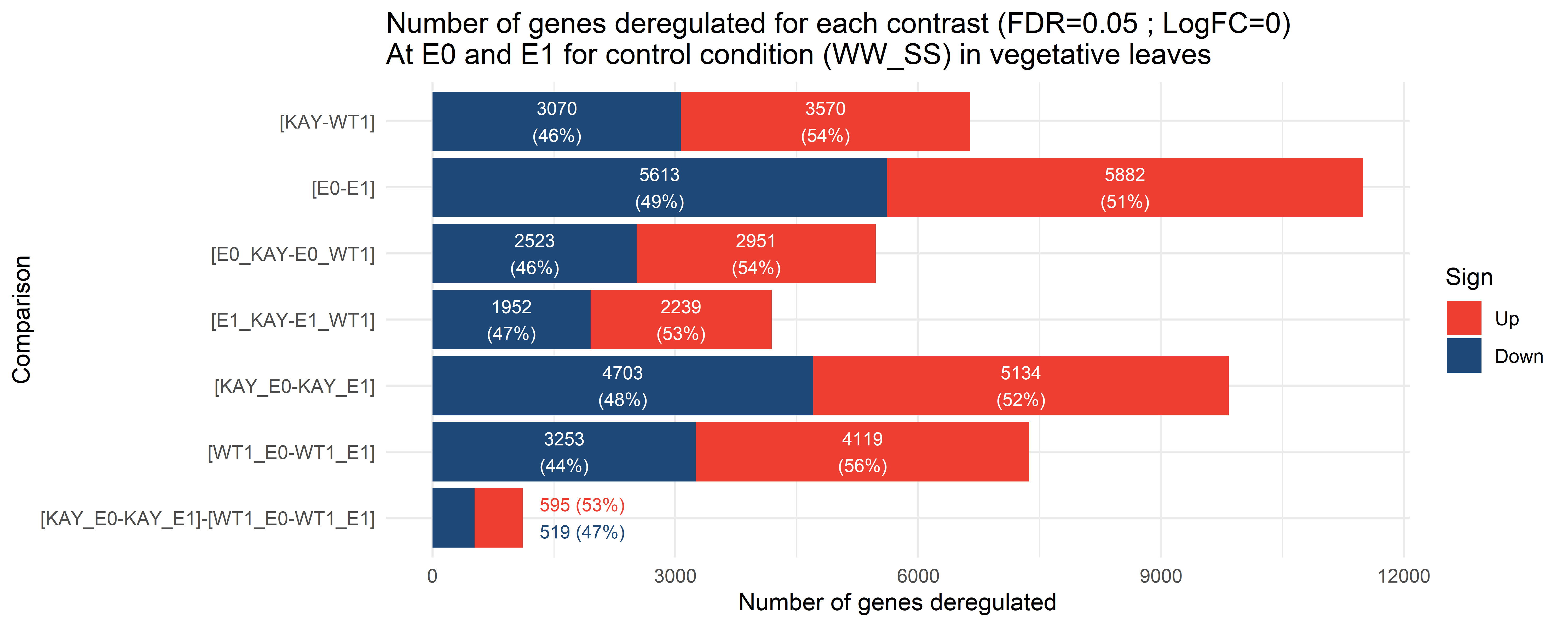 ### GO 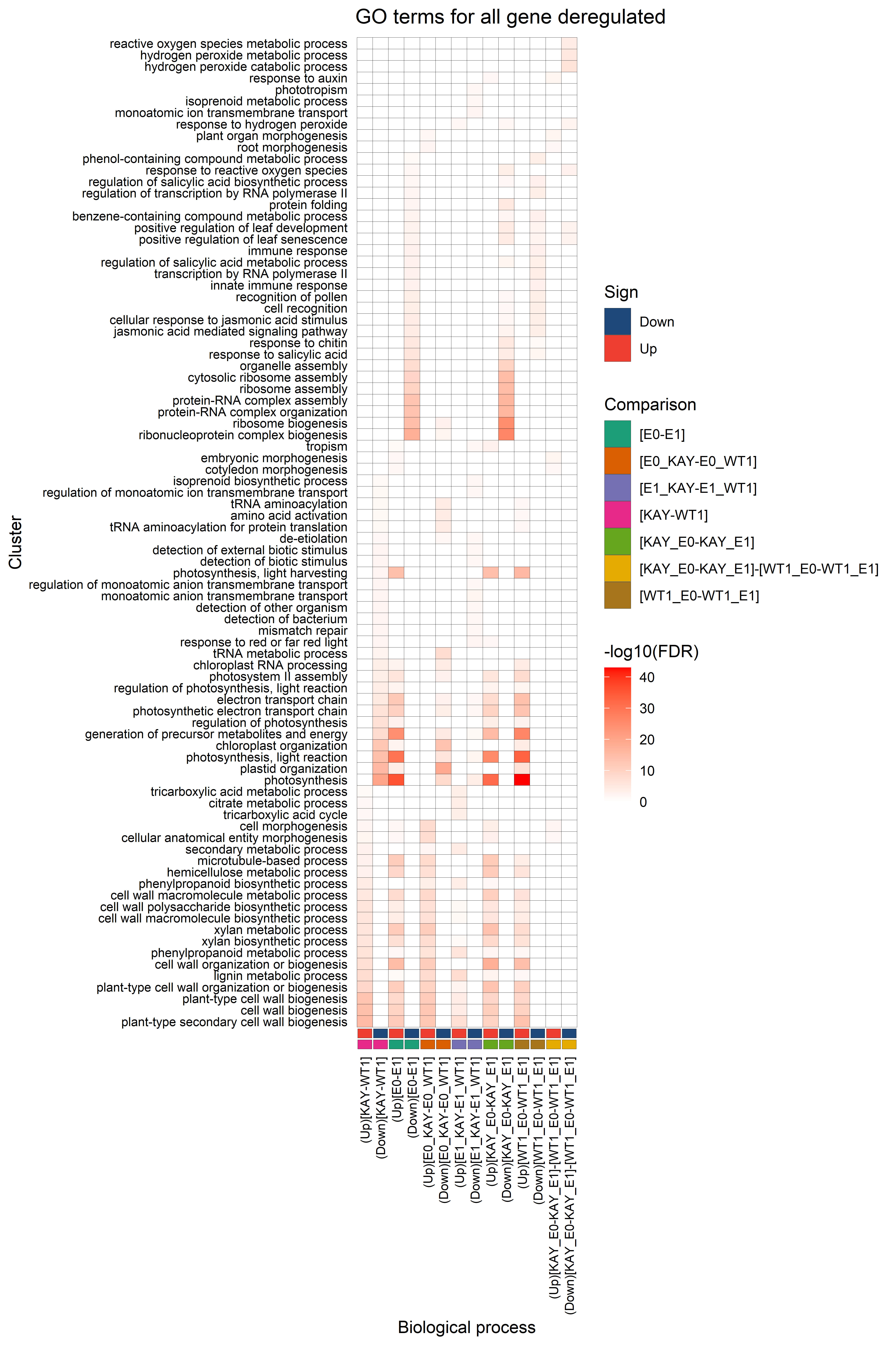 ## Root ### Barplot 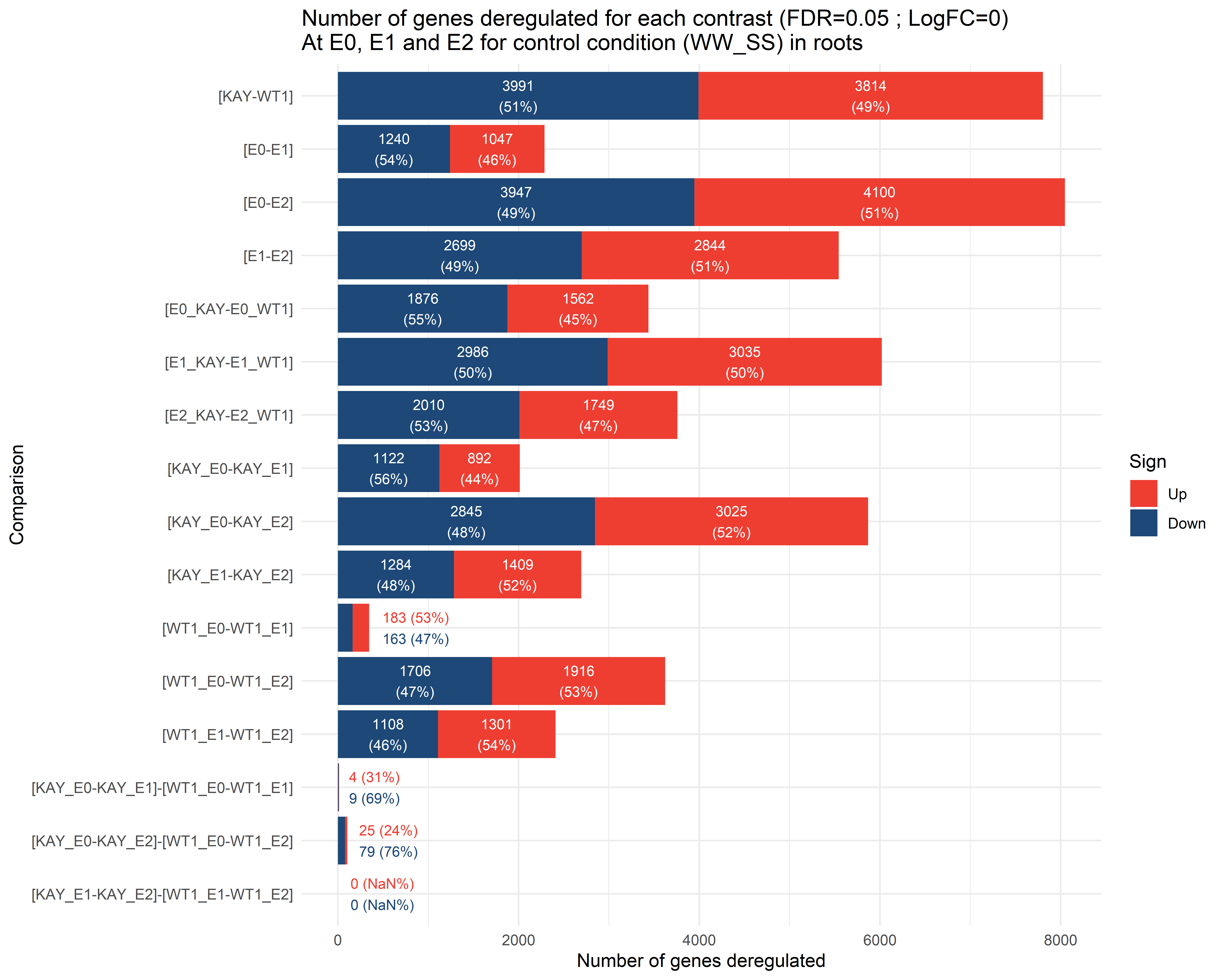 ### GO 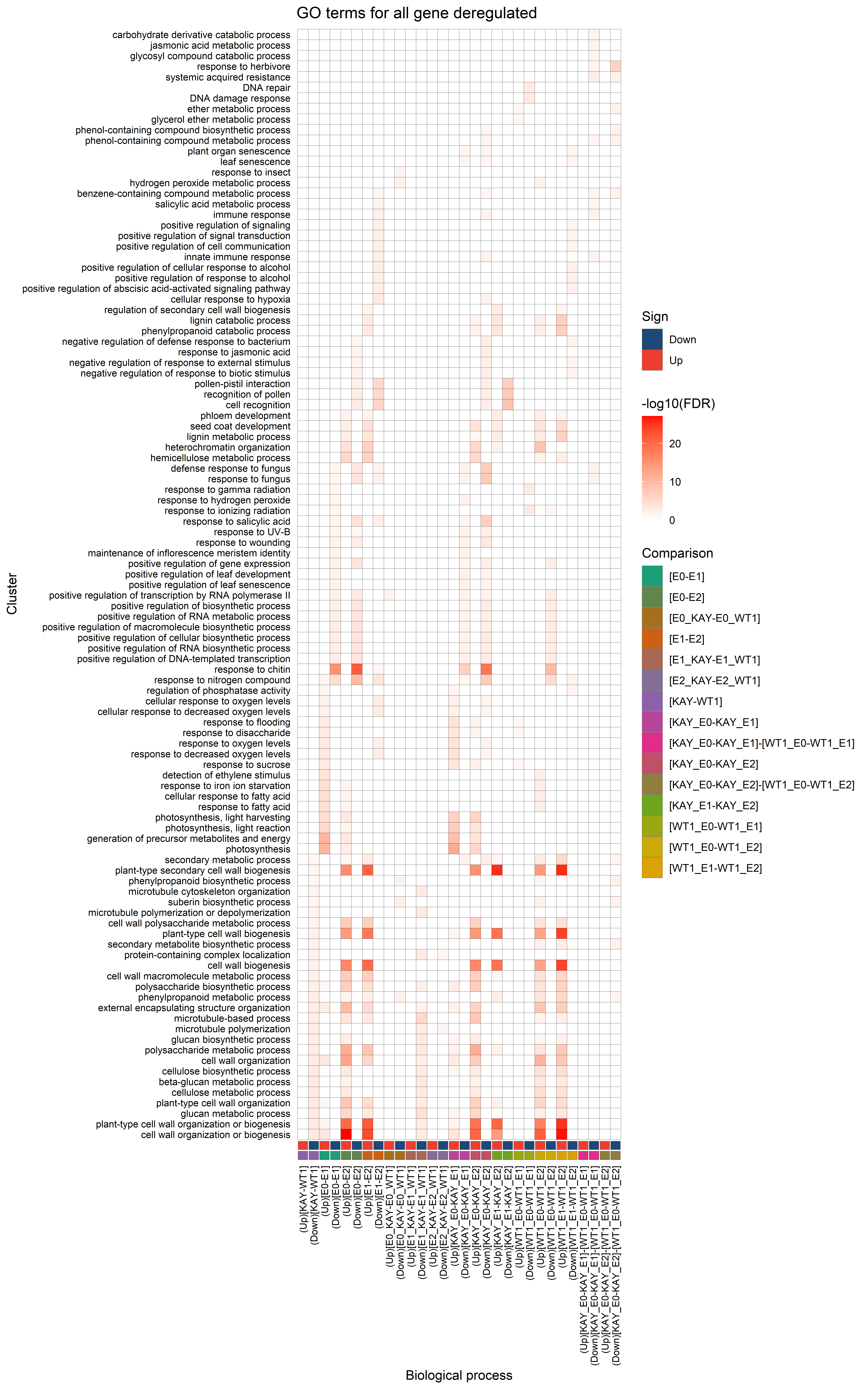 ### Venn diagram of each compartment ```{r, eval = F} #parameter lfc_lim_i = 0 pval_i =0.05 # Data importation load(file = here::here(paste0("data/rnaseq/output/genotype_compartment_effect/contraste_lfc_",lfc_lim_i,"_E0_E1_WW_SS_VL.RData"))) res_list_E0_E1_VL = res_list names(res_list_E0_E1_VL) <- paste0(names(res_list_E0_E1_VL), "(VL)") load(file = here::here(paste0("data/rnaseq/output/genotype_compartment_effect/contraste_lfc_",lfc_lim_i,"_E0_E1_E2_WW_SS_R.RData"))) res_list_E0_E1_E2_R = res_list names(res_list_E0_E1_E2_R) <- paste0(names(res_list_E0_E1_E2_R), "(R)") rm(res_list) names(res_list_E0_E1_VL) p_VL_KAY_VL_WT1<- list( "(Down)[E0_KAY-E0_WT1](VL)" = res_list_E0_E1_VL[["(Down)[E0_KAY-E0_WT1](VL)"]], "(Down)[E1_KAY-E1_WT1](VL)" = res_list_E0_E1_VL[["(Down)[E1_KAY-E1_WT1](VL)"]], "(Up)[E0_KAY-E0_WT1](VL)" = res_list_E0_E1_VL[["(Up)[E0_KAY-E0_WT1](VL)"]], "(Up)[E1_KAY-E1_WT1](VL)" = res_list_E0_E1_VL[["(Up)[E1_KAY-E1_WT1](VL)"]] ) euler_VL_KAY_VL_WT1 <- plot(eulerr::euler(p_VL_KAY_VL_WT1, shape = "ellipse"), quantities = TRUE, fills = c(lighten("#1d4877", amount = -.1), lighten(as.character("#1d4877"), amount = .6), lighten("#ee3e32", amount = -.1), lighten("#ee3e32", amount = .6)), legend = list(side = "right"), main = list(label = "\nEuler diagram of down and up regulated genes for \ndifference between KAY and WT1 only for vegetative leaf at E1 and E2", cex = 1.3)) p_R_KAY_R_WT1<- list( "(Down)[E0_KAY-E0_WT1](R)" = res_list_E0_E1_E2_R[["(Down)[E0_KAY-E0_WT1](R)"]], "(Down)[E1_KAY-E1_WT1](R)" = res_list_E0_E1_E2_R[["(Down)[E1_KAY-E1_WT1](R)"]], "(Down)[E2_KAY-E2_WT1](R)" = res_list_E0_E1_E2_R[["(Down)[E2_KAY-E2_WT1](R)"]], "(Up)[E0_KAY-E0_WT1](R)" = res_list_E0_E1_E2_R[["(Up)[E0_KAY-E0_WT1](R)"]], "(Up)[E1_KAY-E1_WT1](R)" = res_list_E0_E1_E2_R[["(Up)[E1_KAY-E1_WT1](R)"]], "(Up)[E2_KAY-E2_WT1](R)" = res_list_E0_E1_E2_R[["(Up)[E2_KAY-E1_WT2](R)"]] ) euler_R_KAY_R_WT1 <- plot(eulerr::euler(p_R_KAY_R_WT1, shape = "ellipse"), quantities = TRUE, fills = c(lighten("#1d4877", amount = -.1), lighten(as.character("#1d4877"), amount = .4),lighten(as.character("#1d4877"), amount = .8), lighten("#ee3e32", amount = -.1), lighten("#ee3e32", amount = .4), lighten("#ee3e32", amount = .8)), legend = list(side = "right"), main = list(label = "Euler diagram of down and up regulated genes for \ndifference between KAY and WT1 only for root at E1 and E2", cex = 1.3)) fig_export(path = here::here(paste0("report/rnaseq/plot/genotype_compartment_effect/euler_VL_lfc_",lfc_lim_i, "_E0_E1_VL")), euler_VL_KAY_VL_WT1, height = 6, width = 8, res_i = 600, format = "png") fig_export(path = here::here(paste0("report/rnaseq/plot/genotype_compartment_effect/euler_R_lfc_",lfc_lim_i, "_E0_E1_E2_R")), euler_R_KAY_R_WT1, height = 6, width = 8, res_i = 600, format = "png") ```