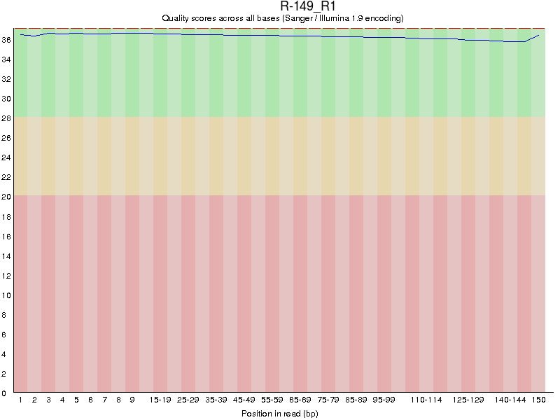
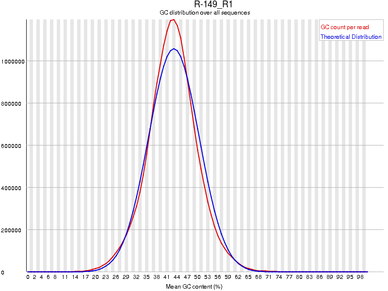
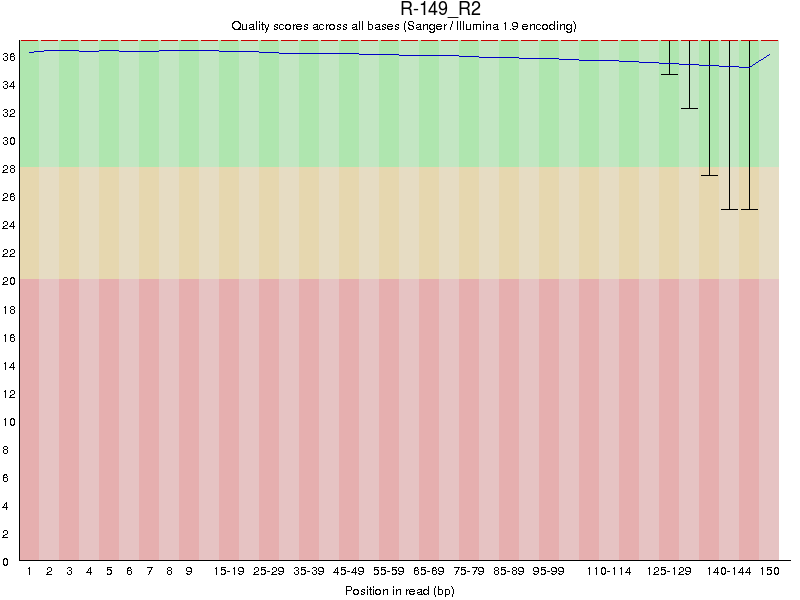
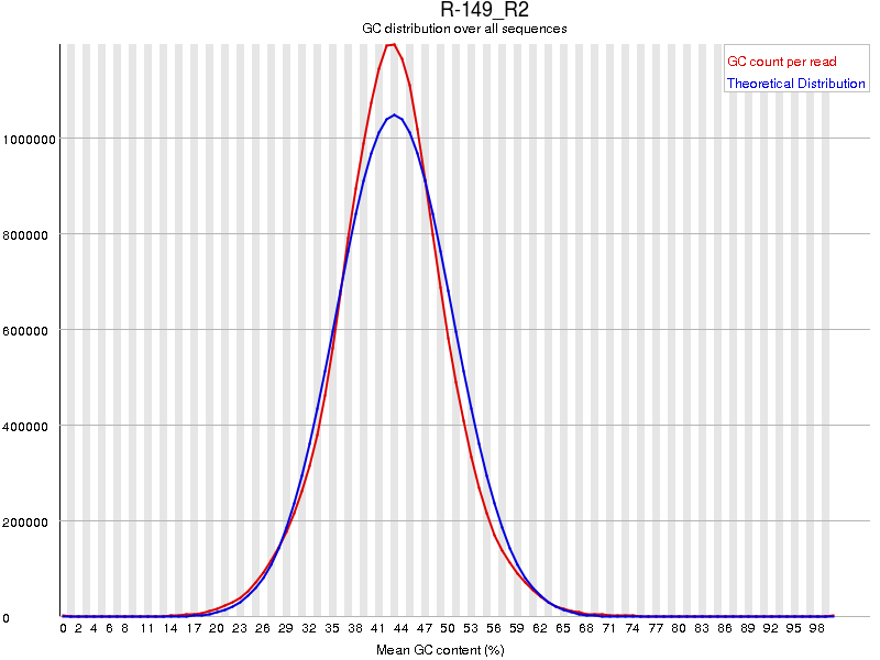
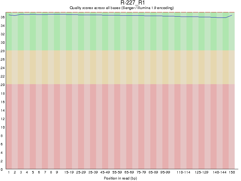
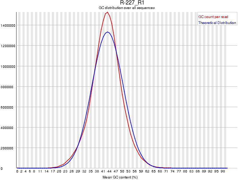
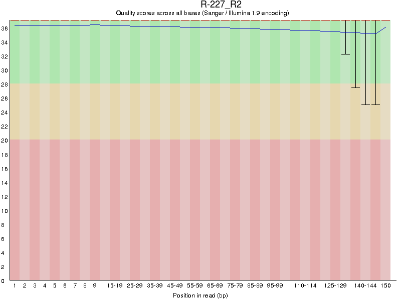
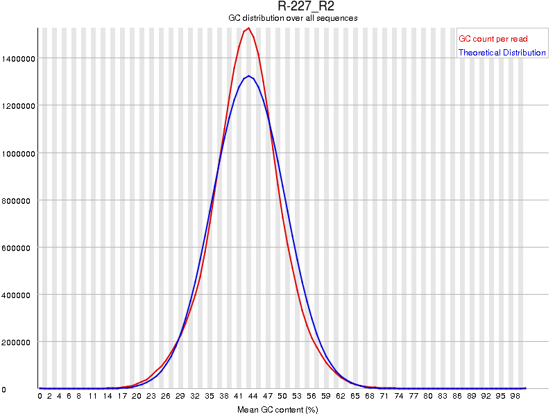
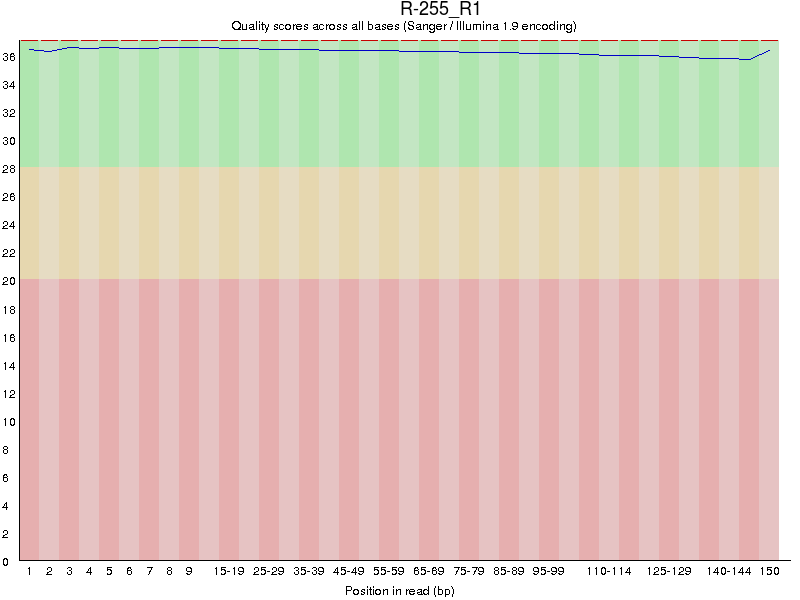
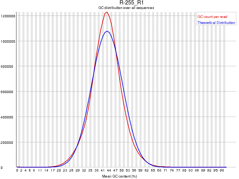
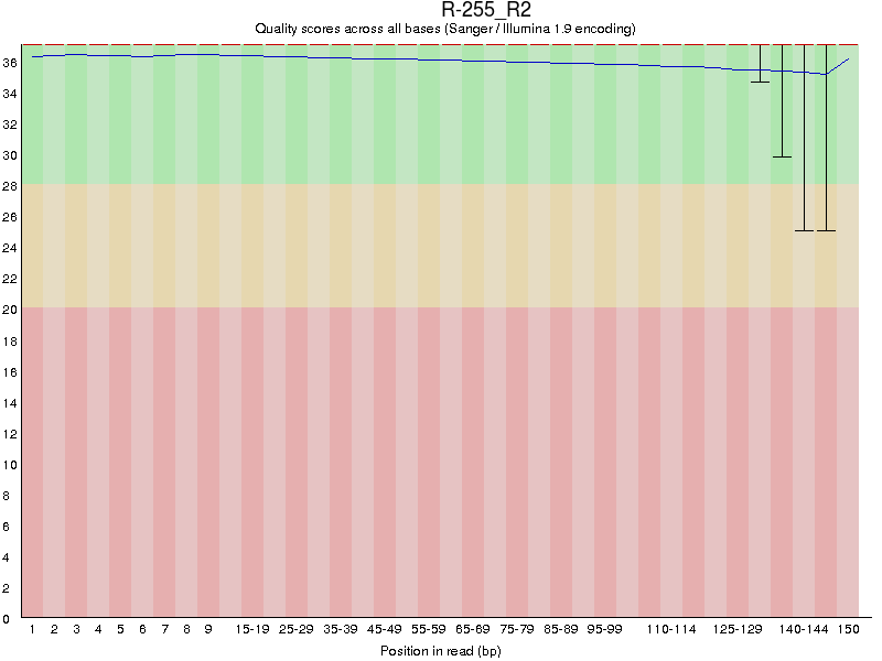
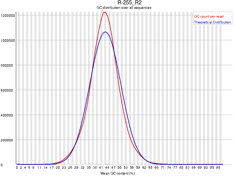
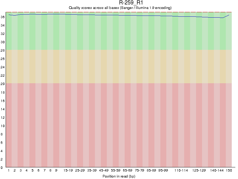
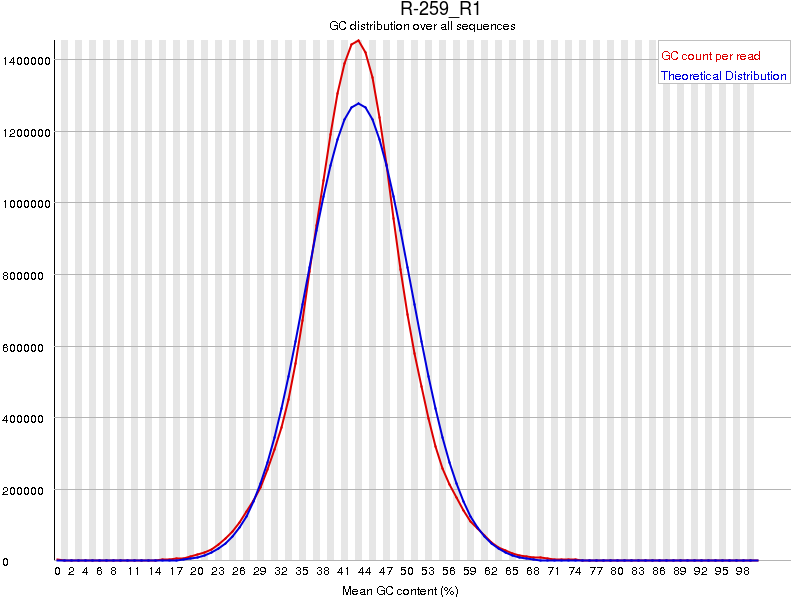
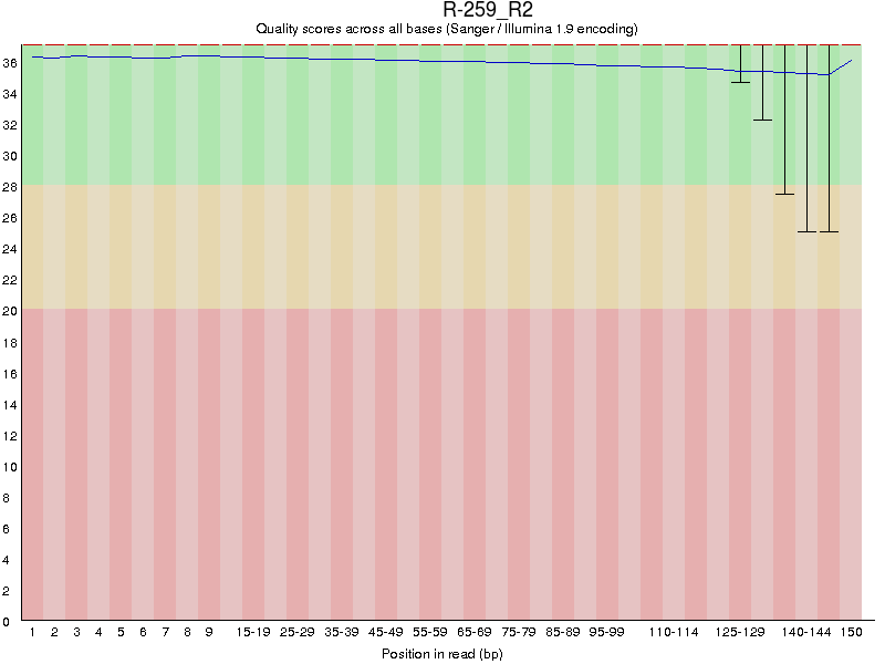
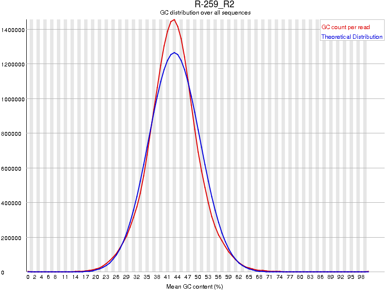
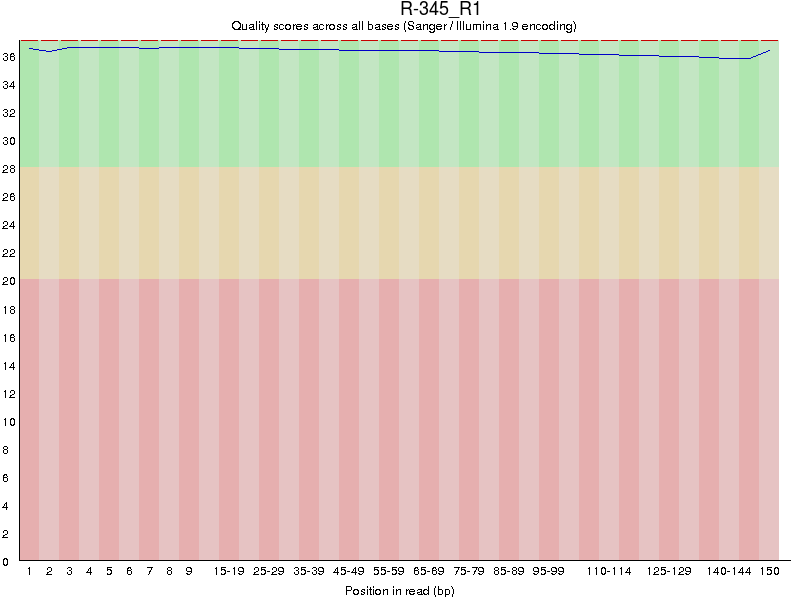
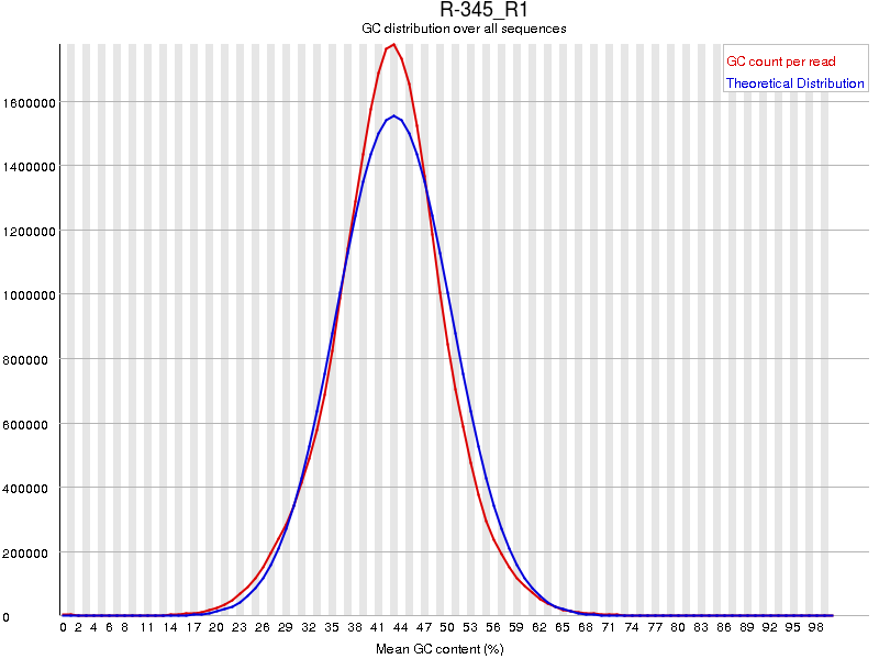
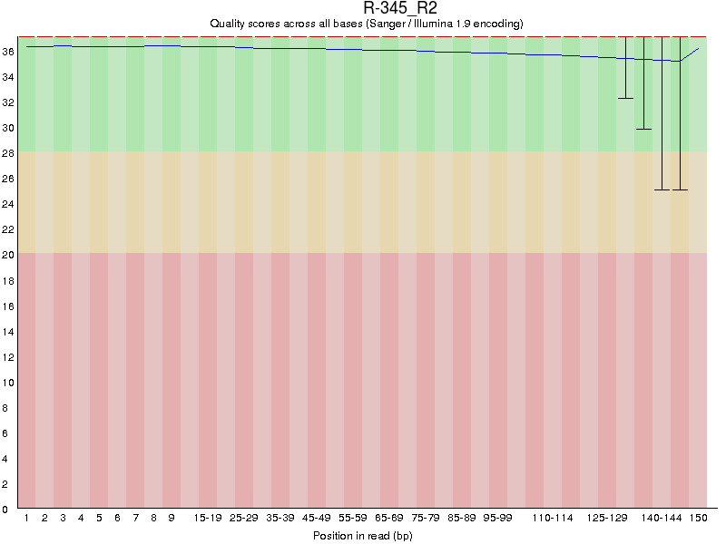
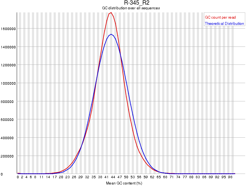
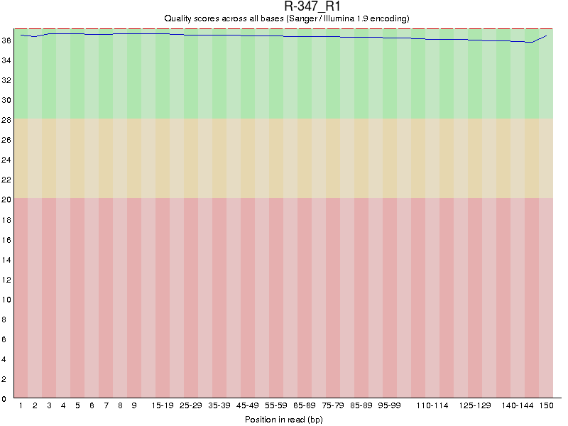
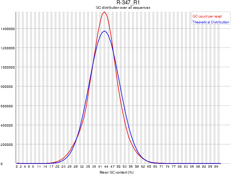
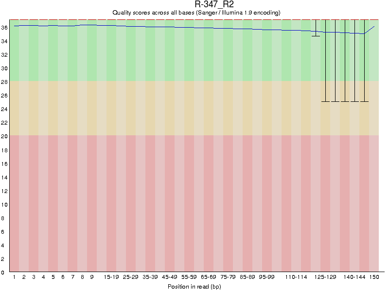
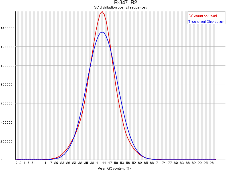
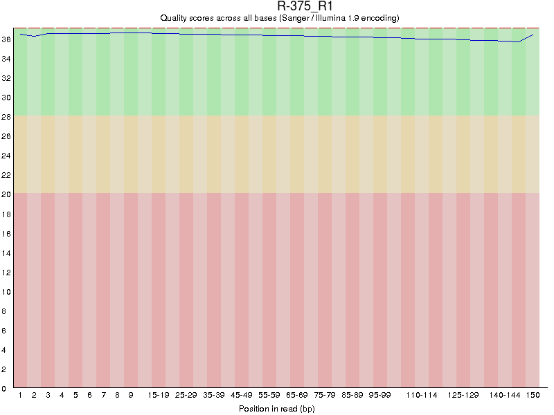
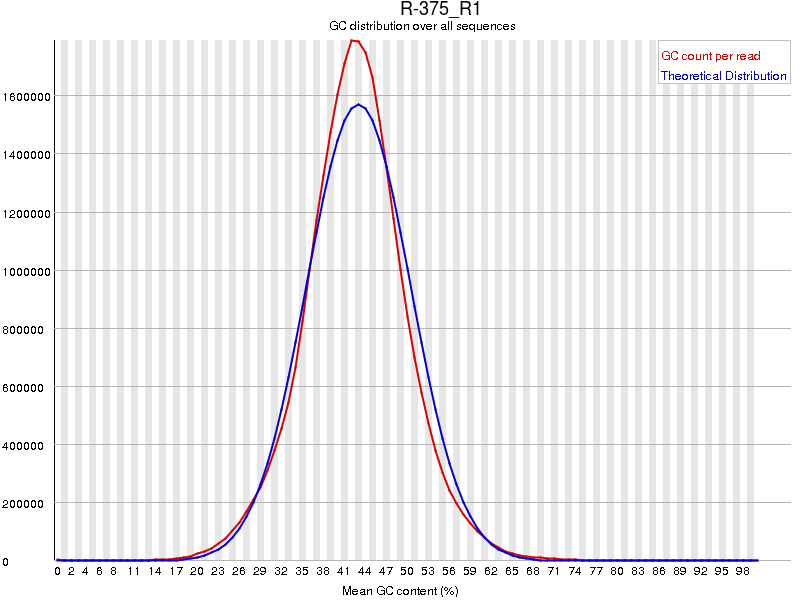
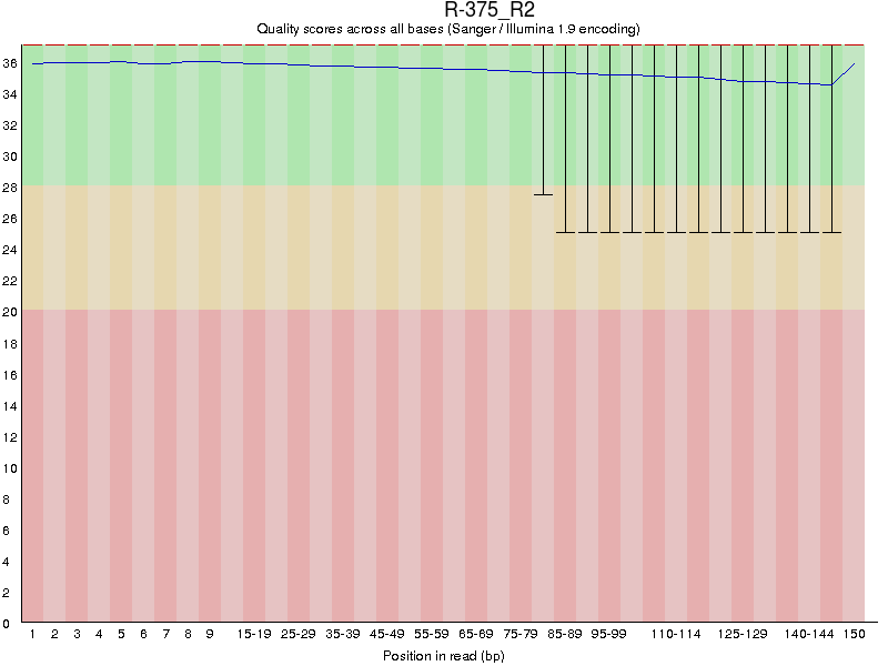
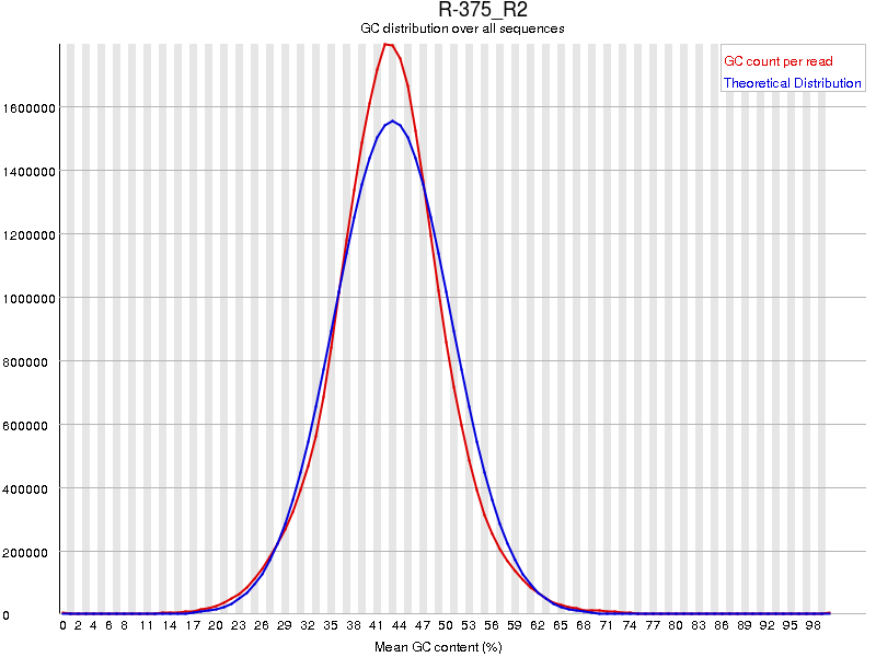
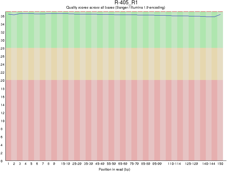
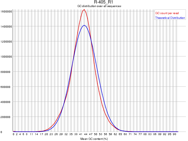
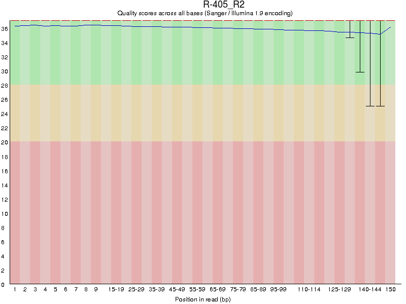
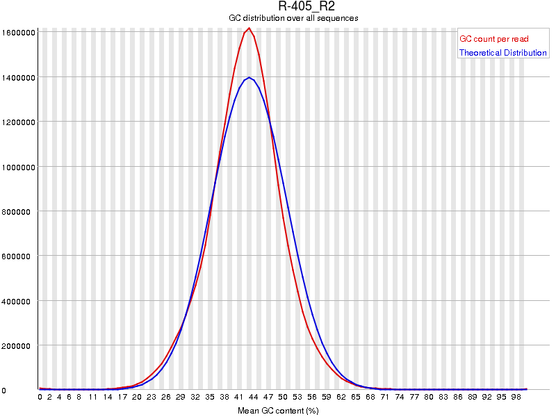
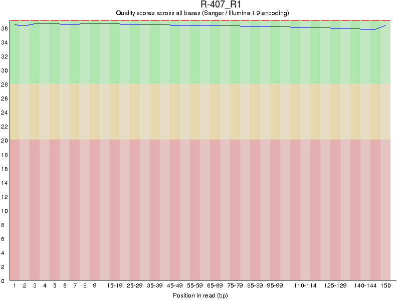
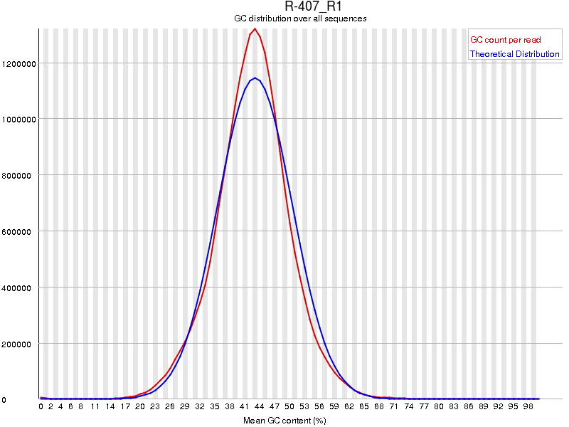
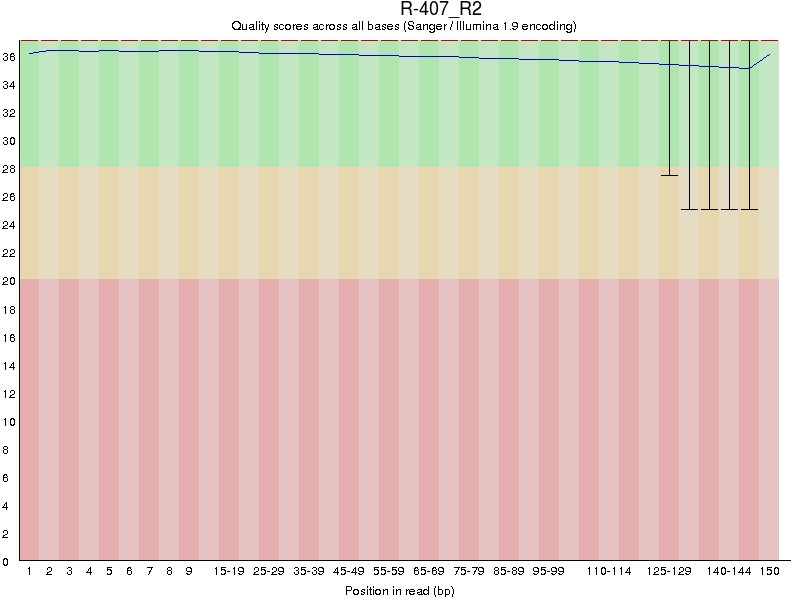
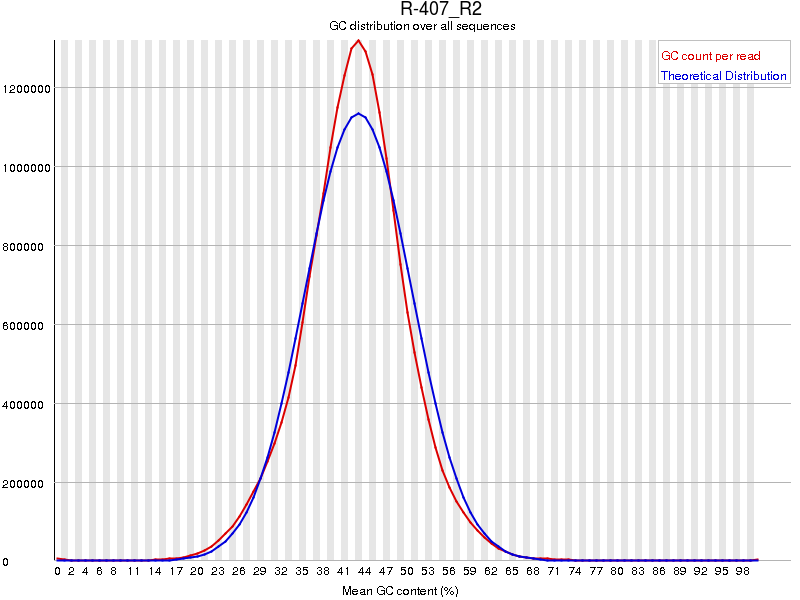
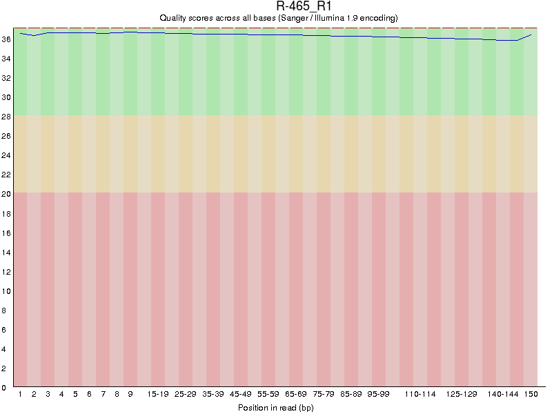
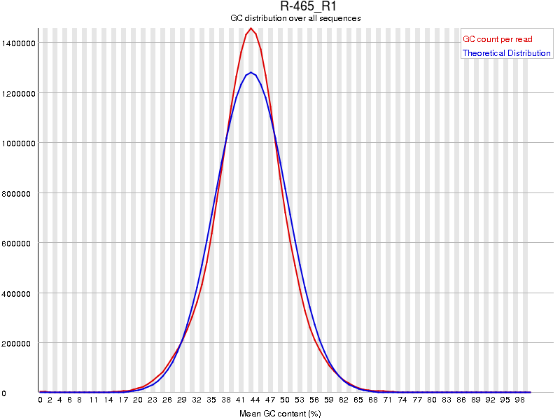
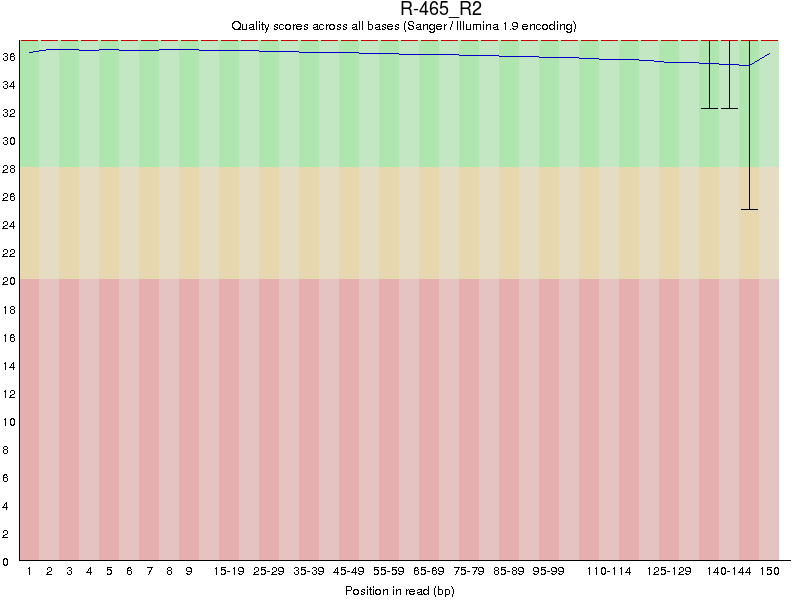
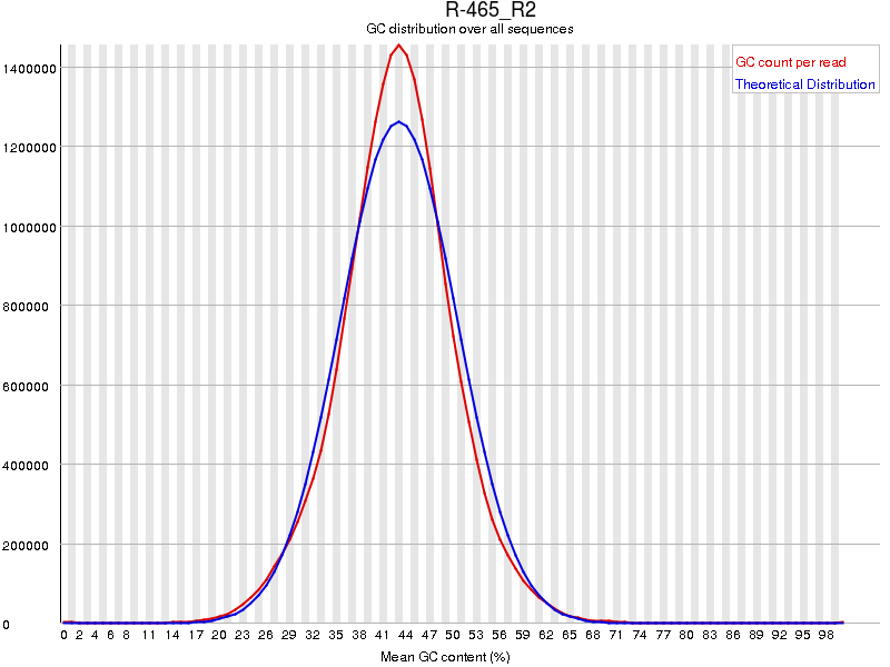
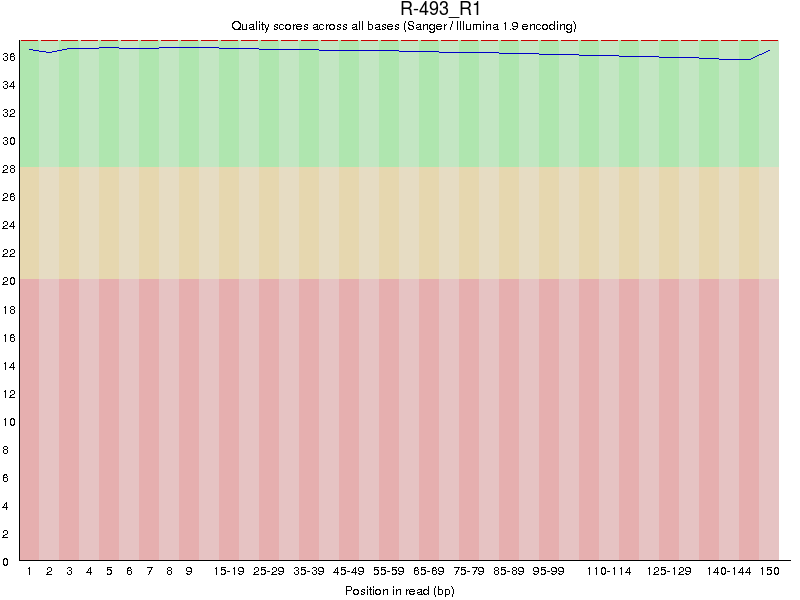
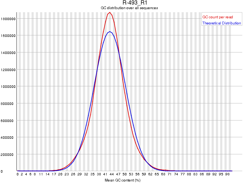
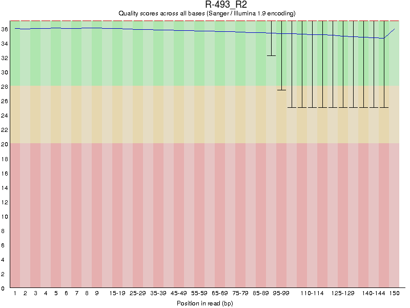
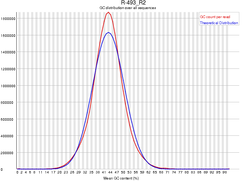
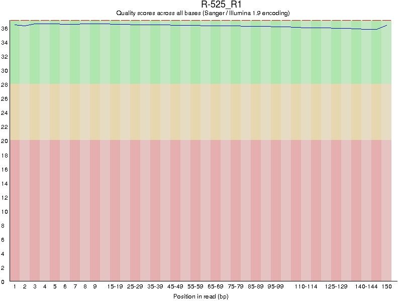
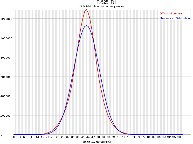
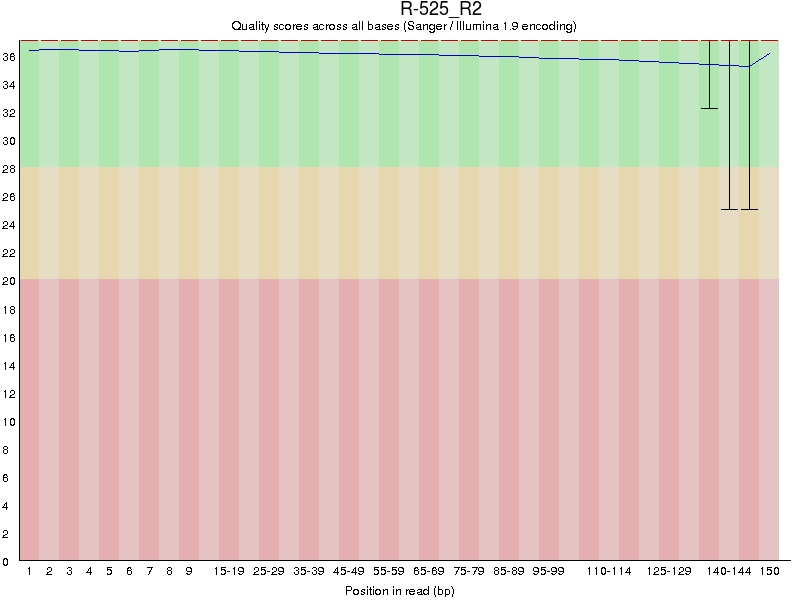
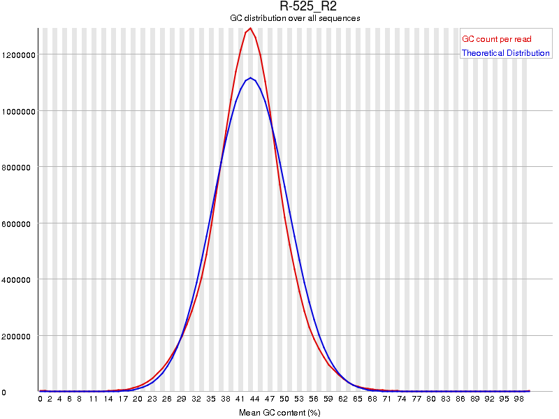
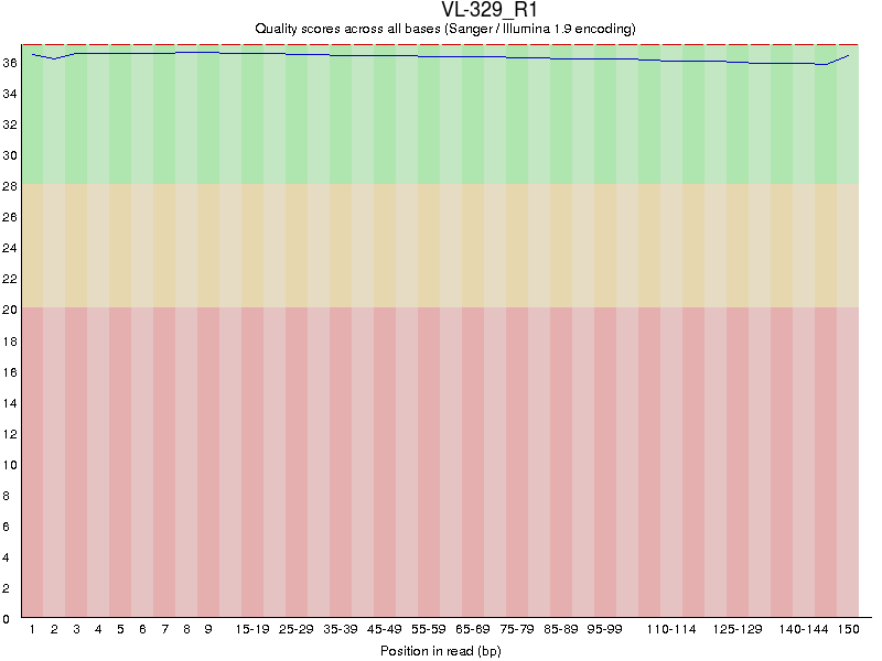
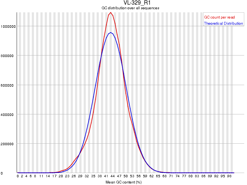
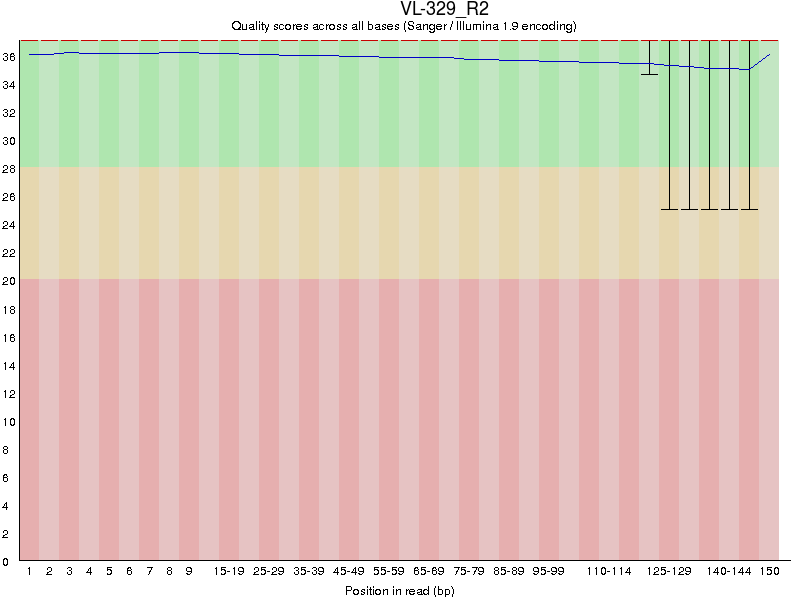
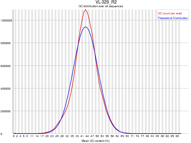
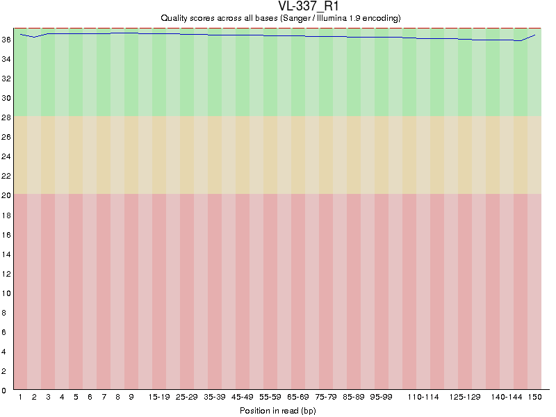
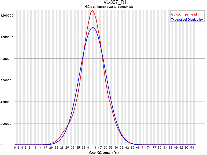
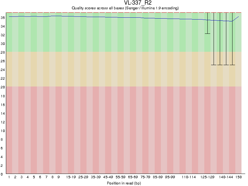
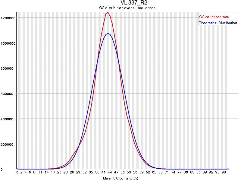
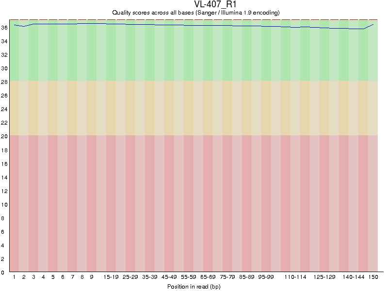
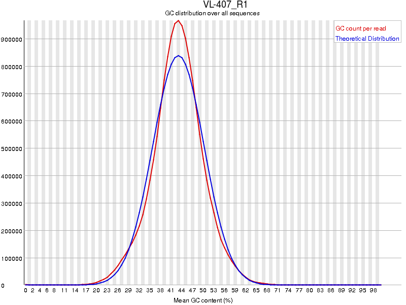
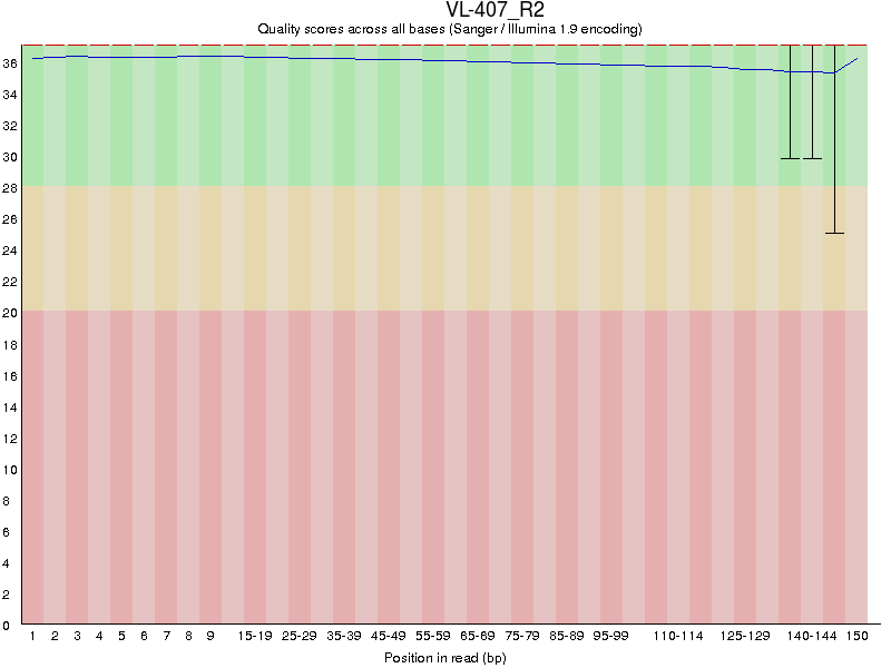
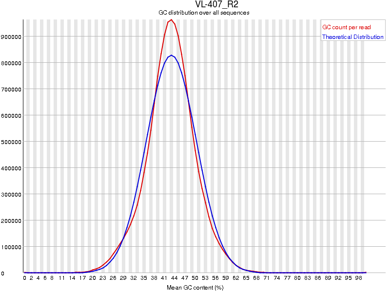
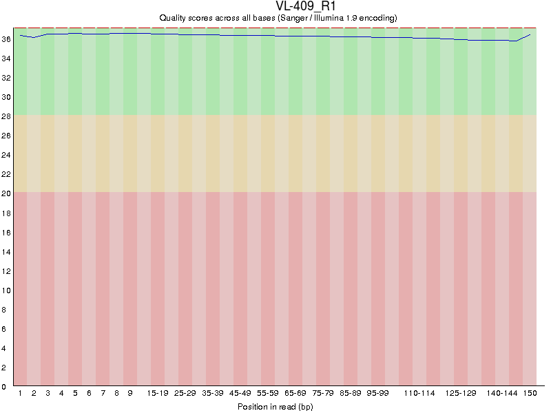
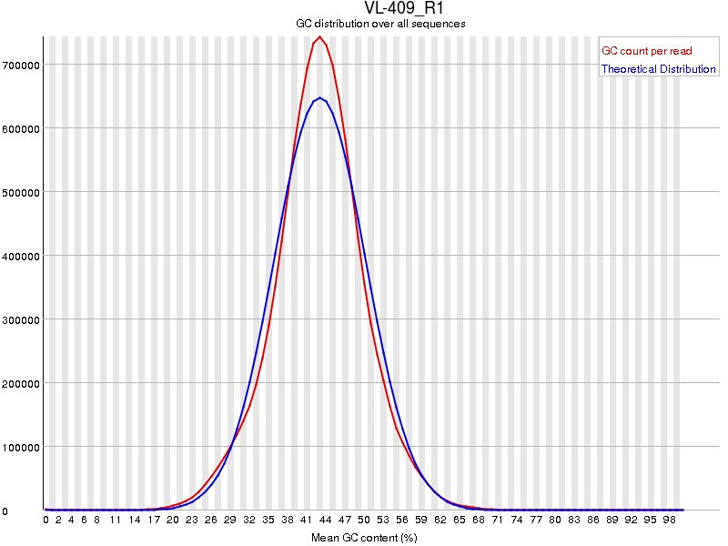
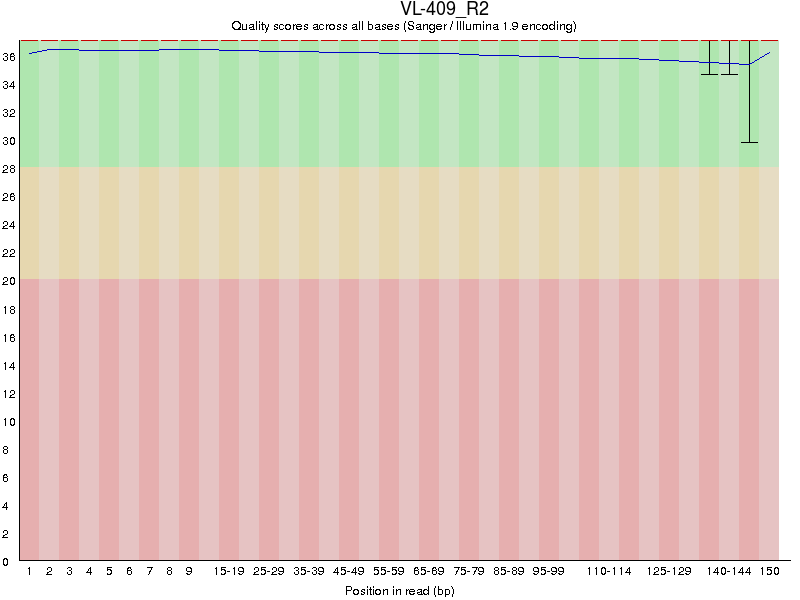
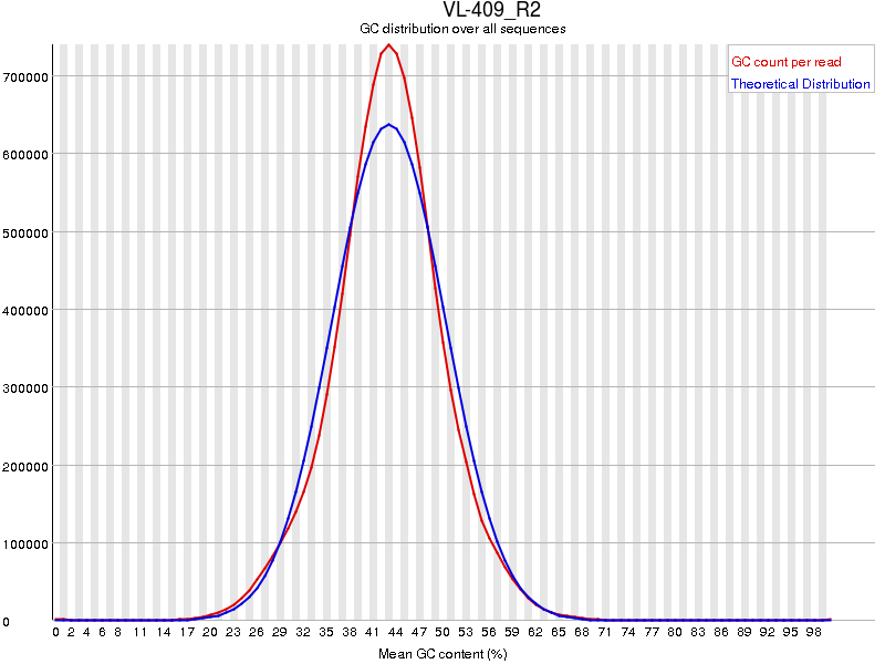
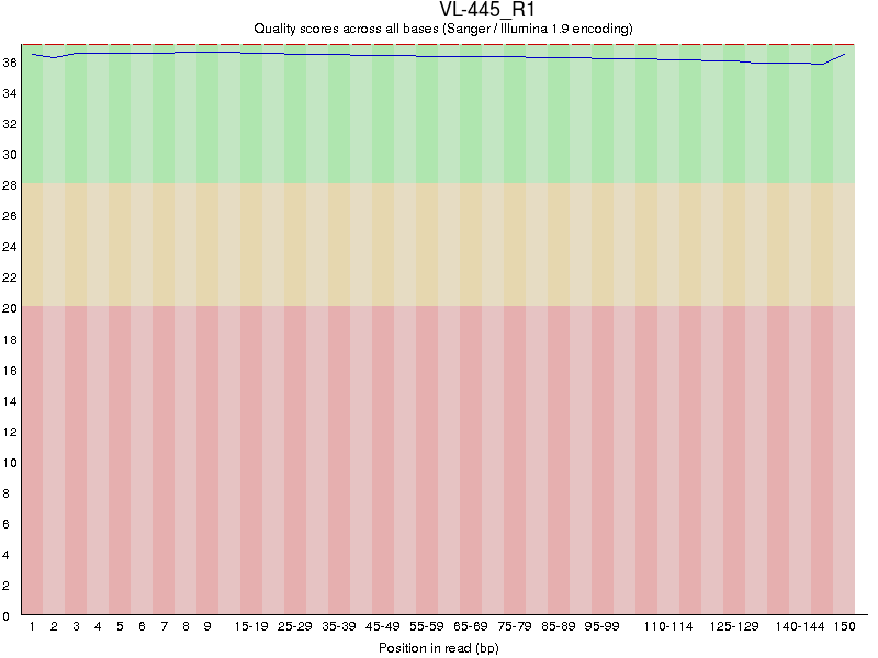
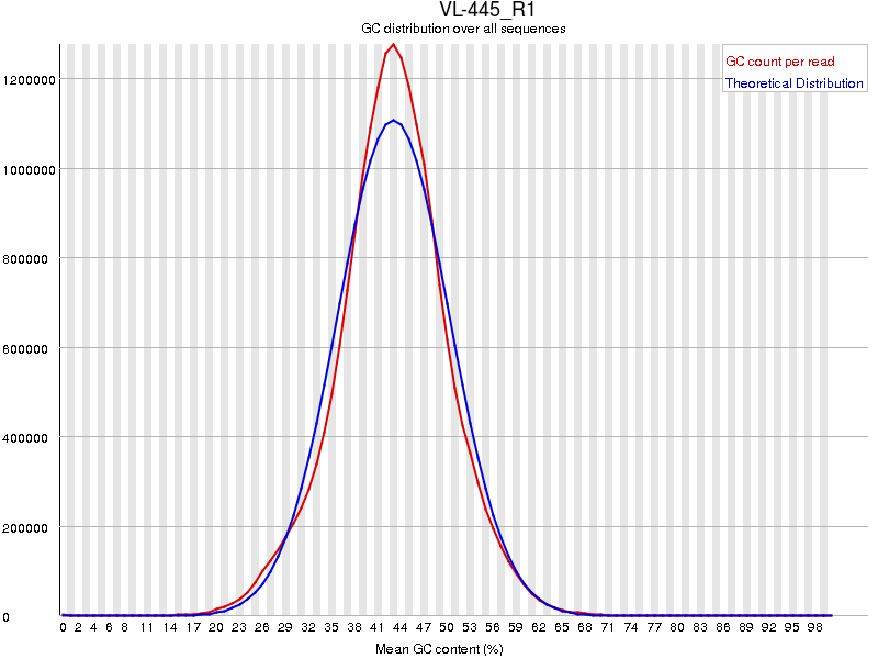
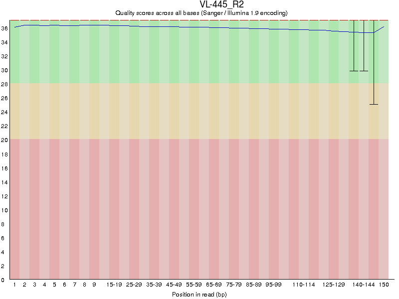
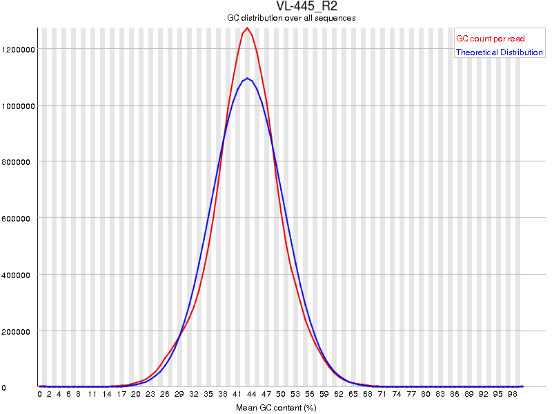
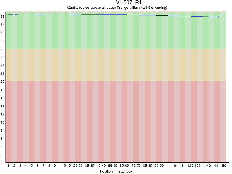
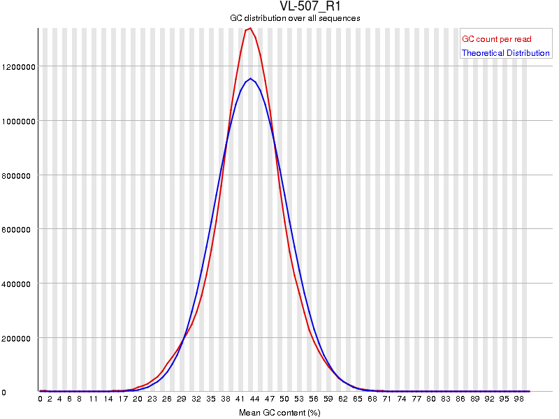
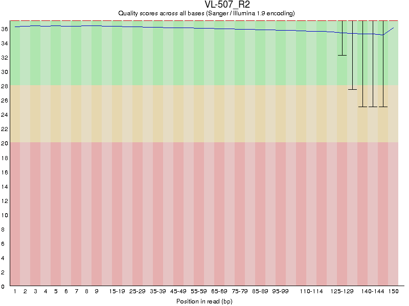
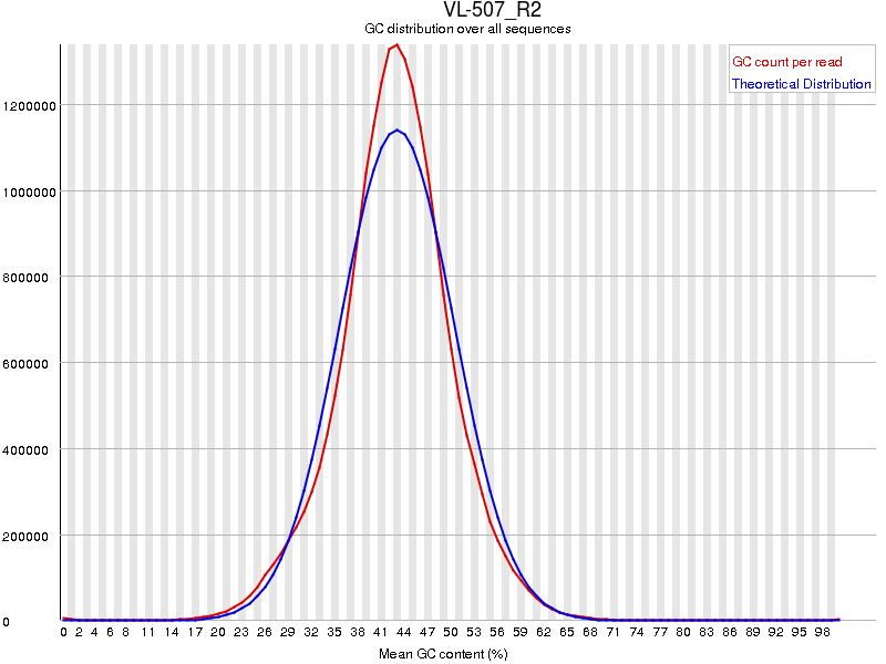
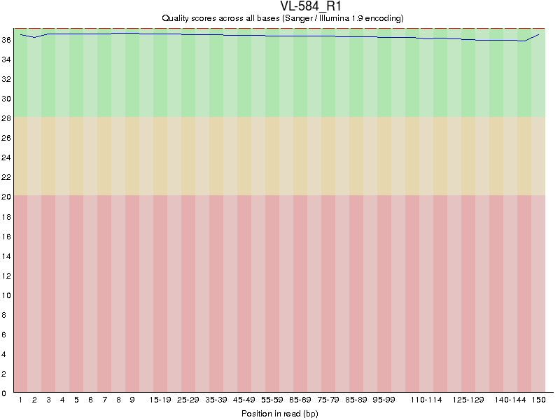
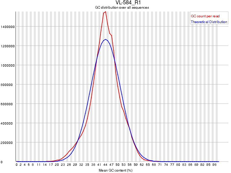
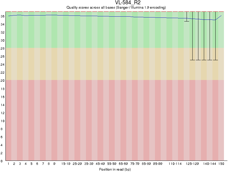
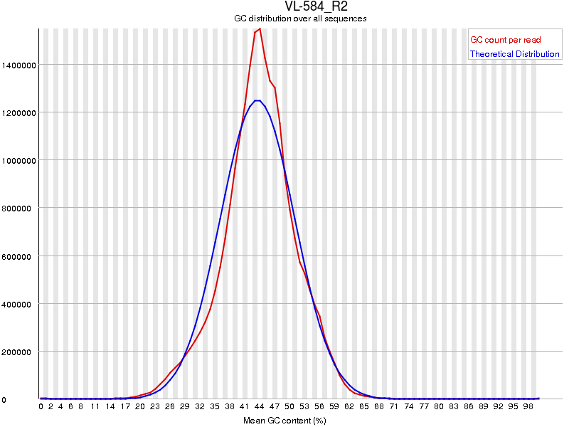
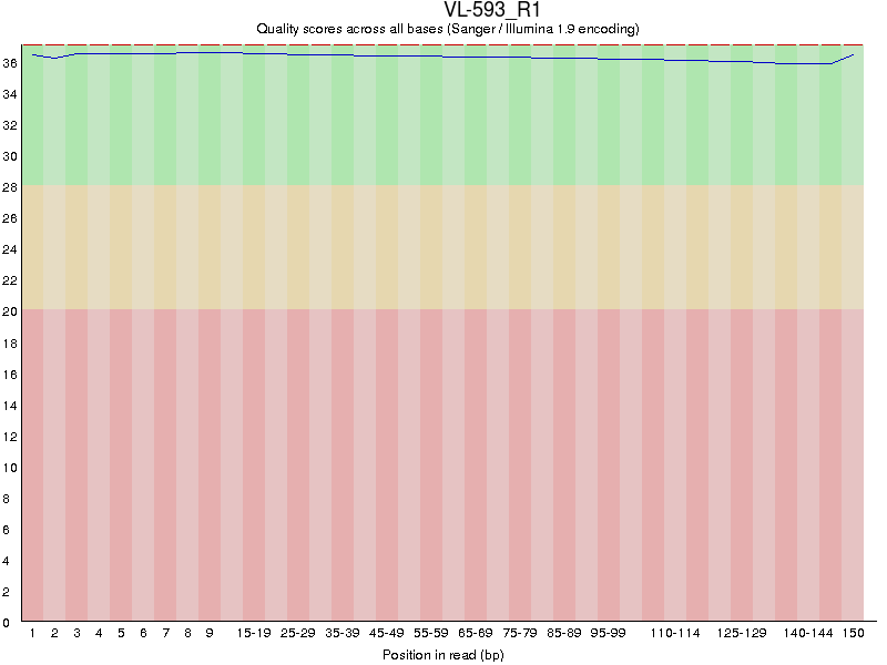
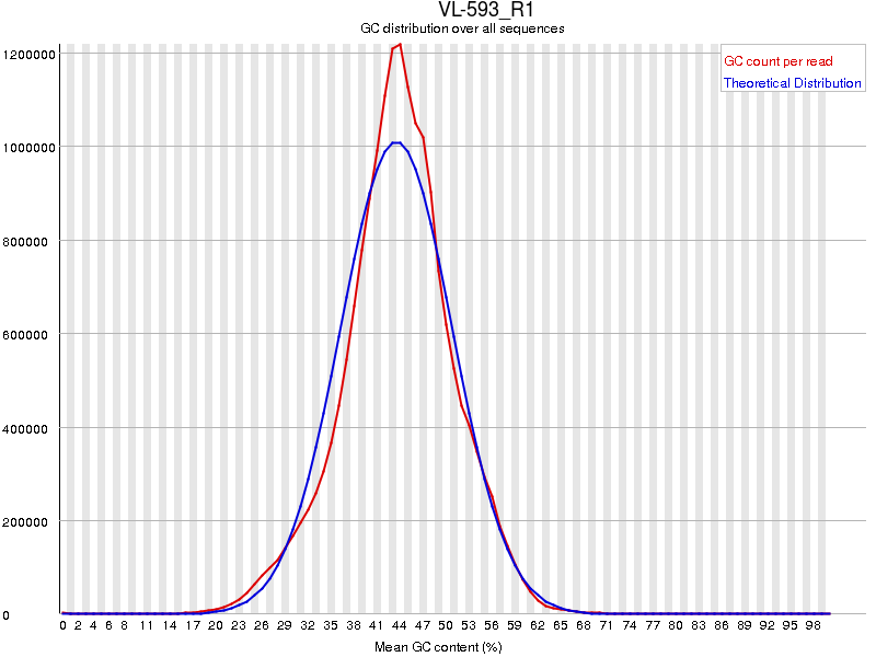
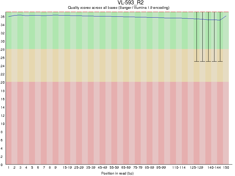
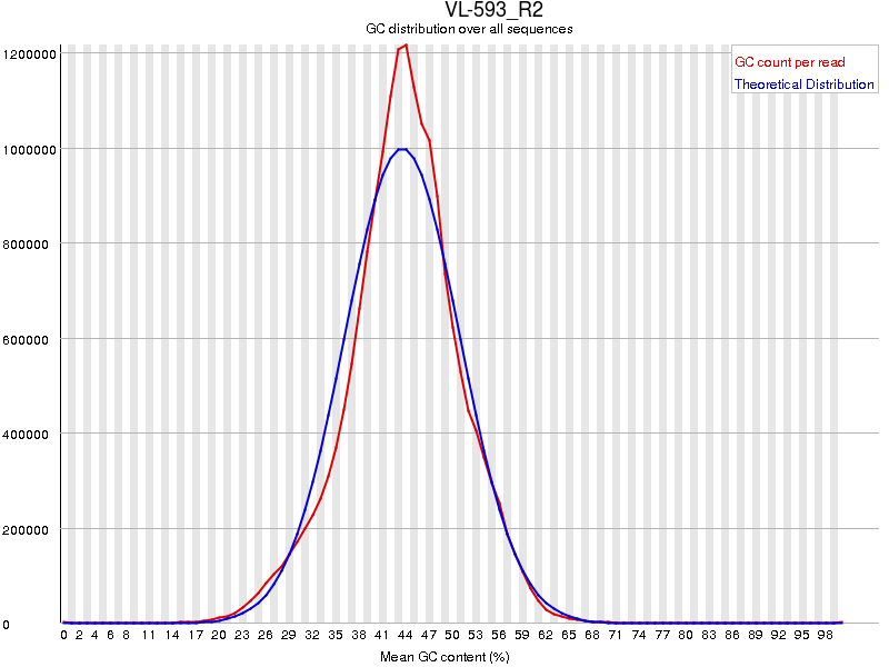
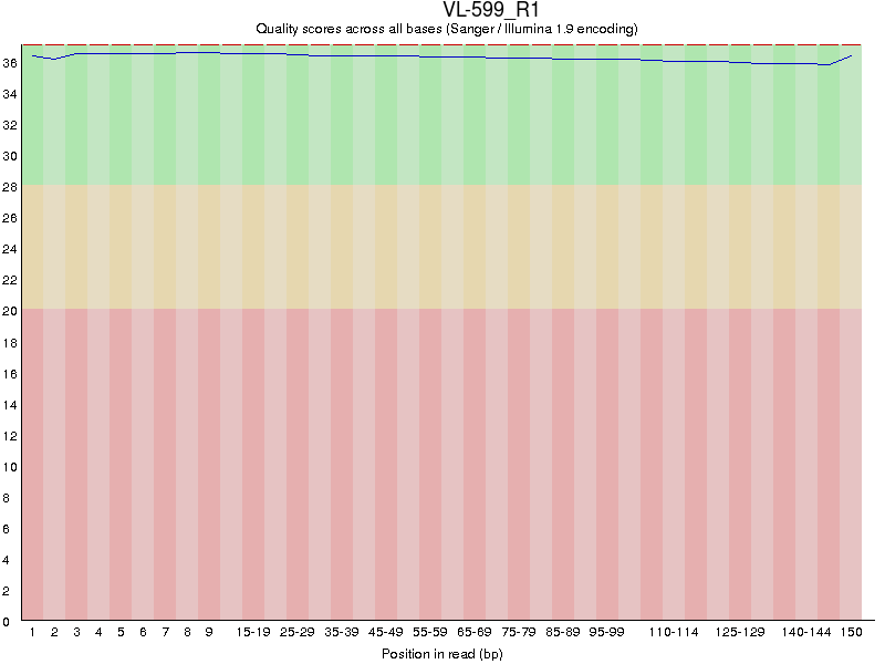
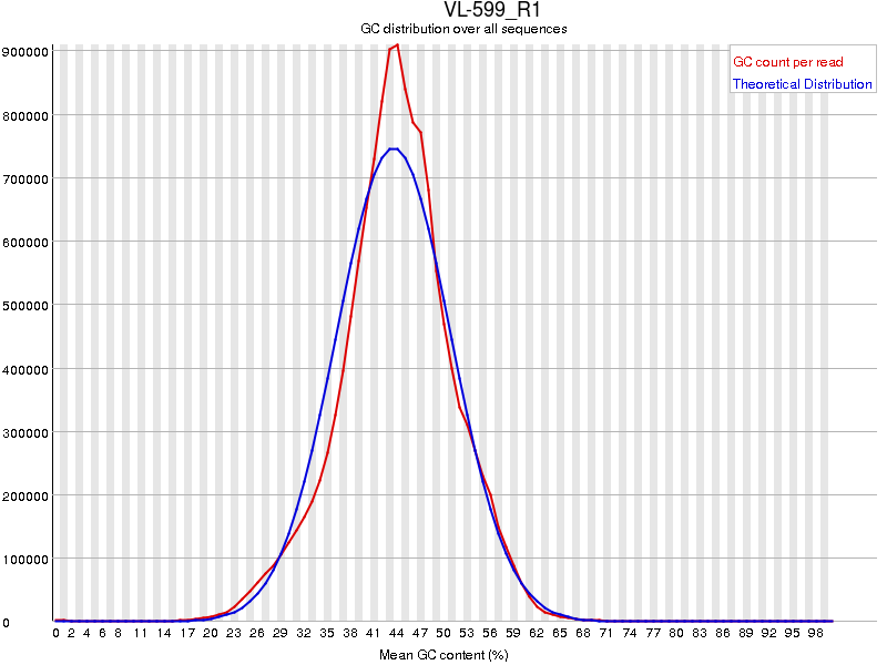
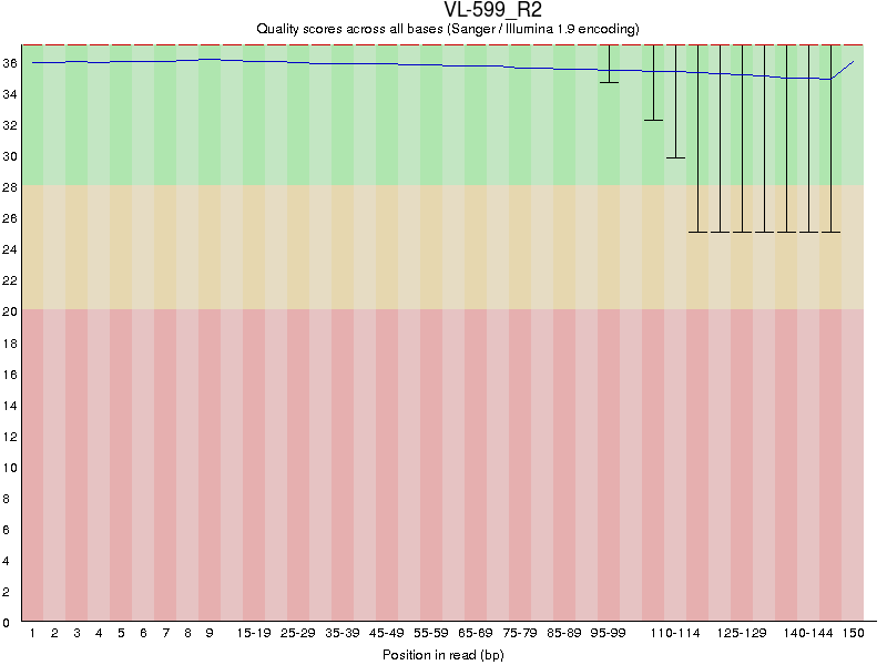
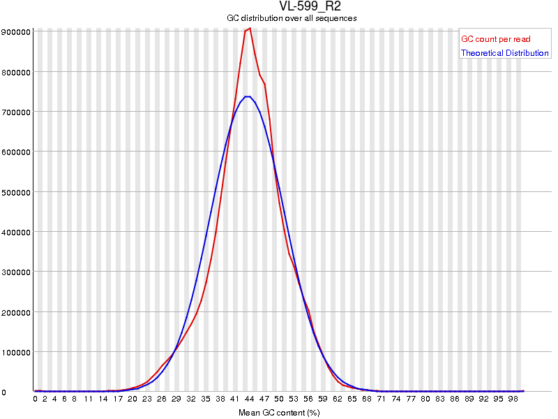
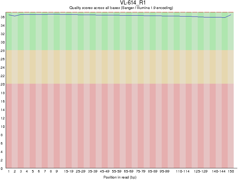
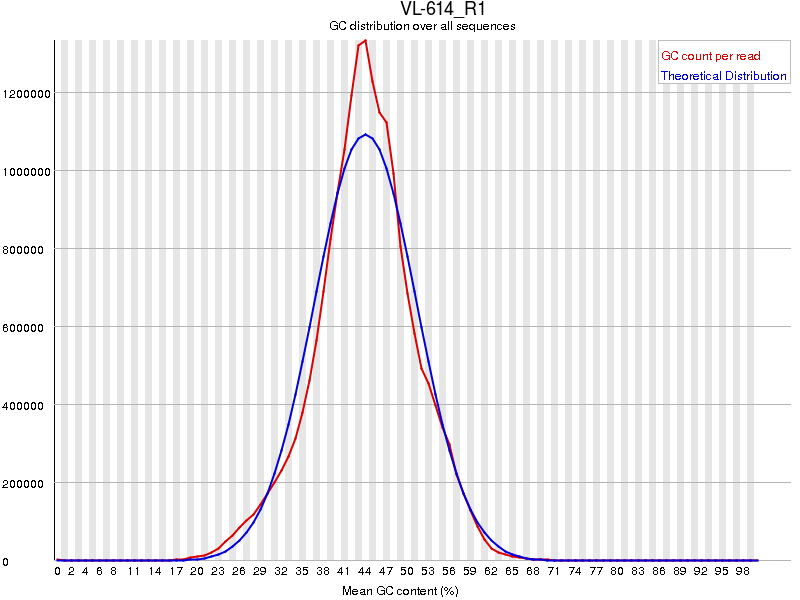
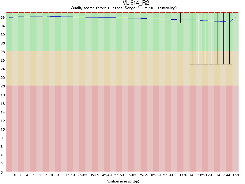
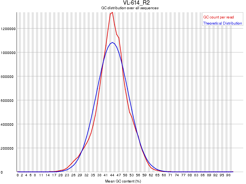
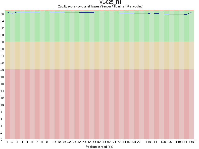
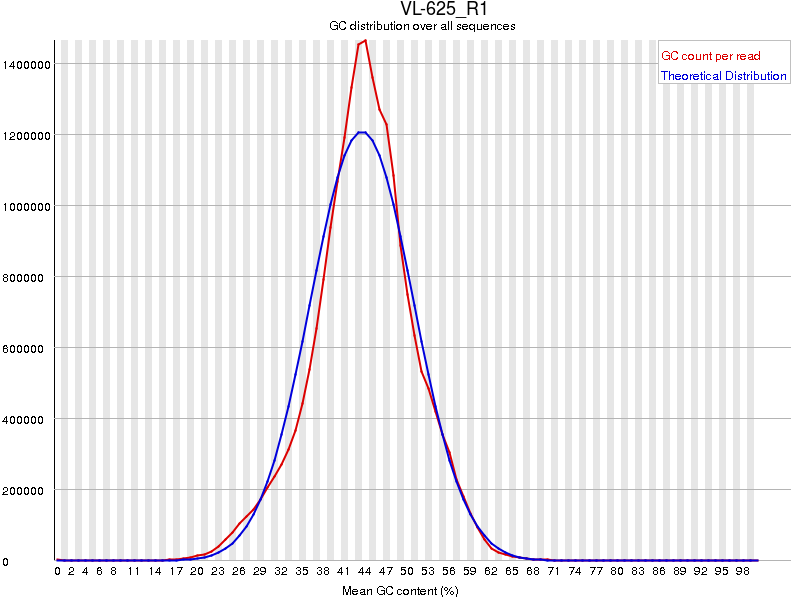
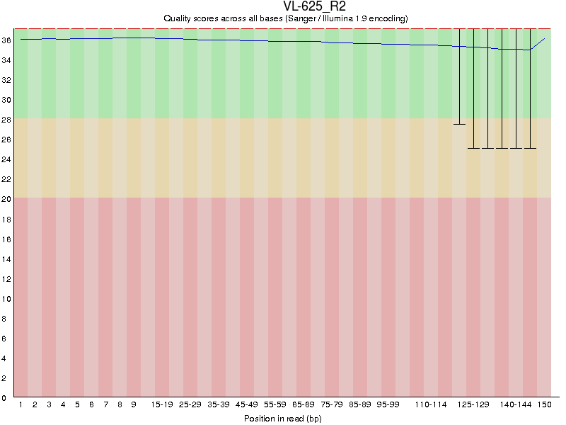
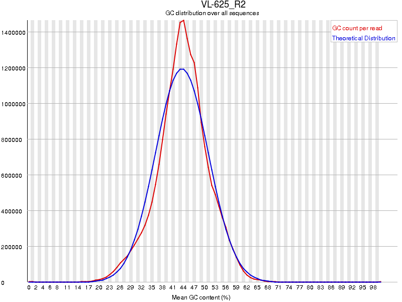
6.3 Mapping sequence reads to the reference genome
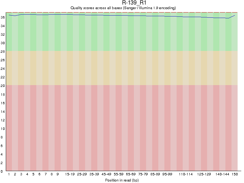
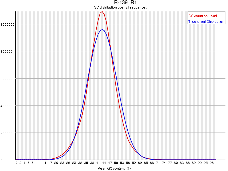
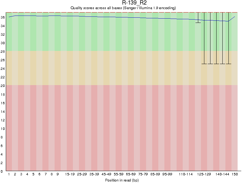
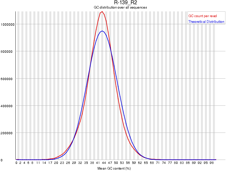
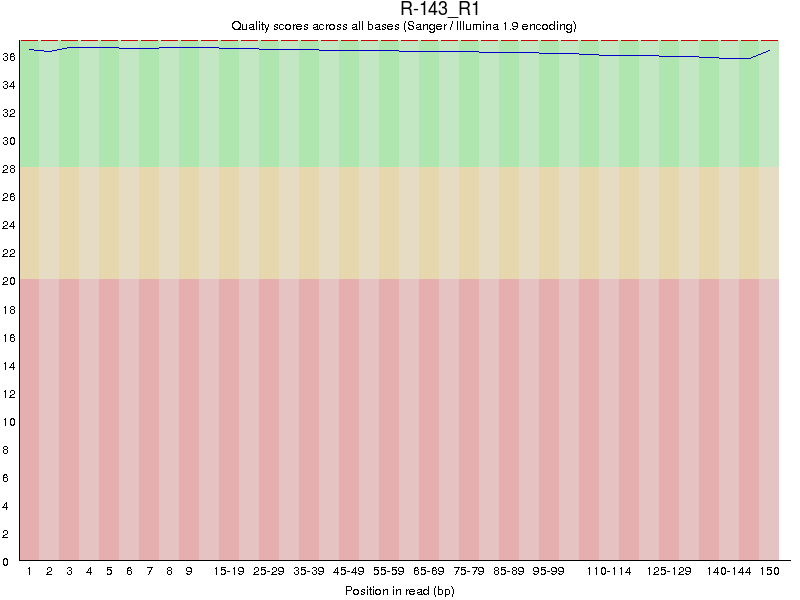
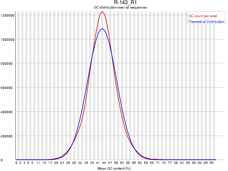
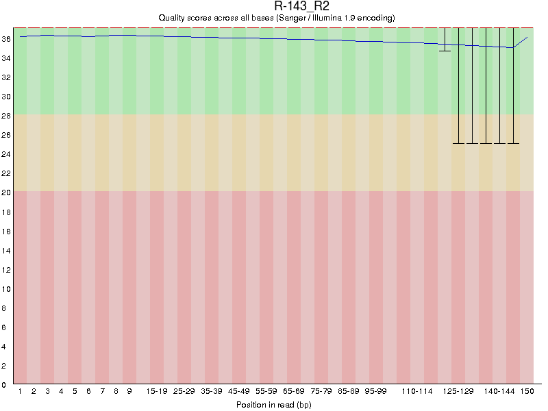
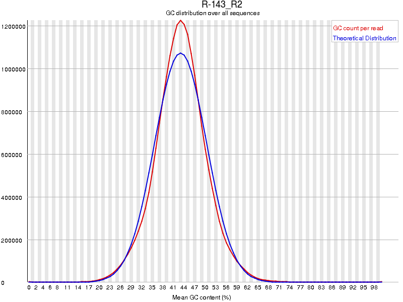
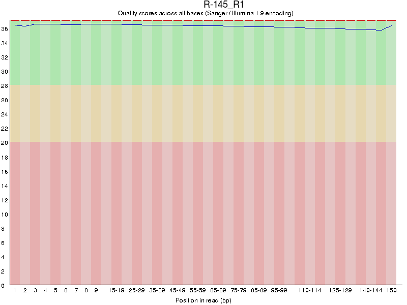
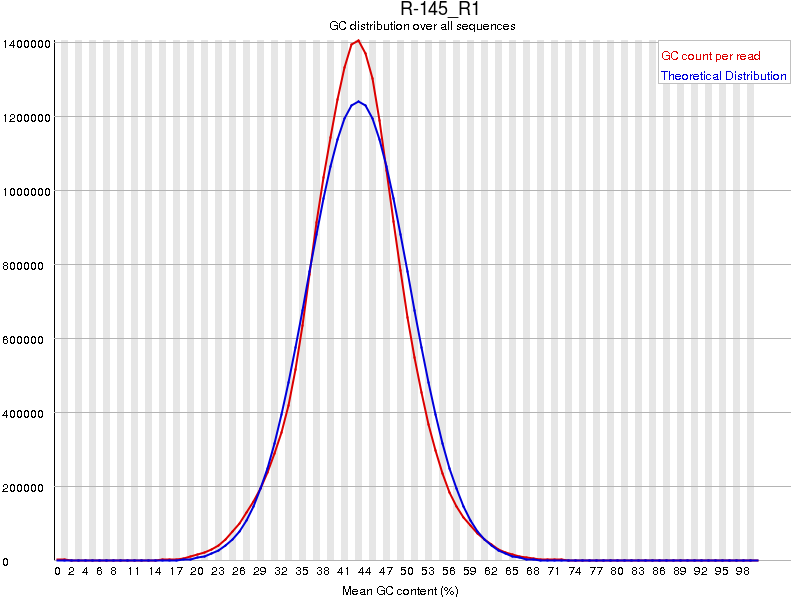
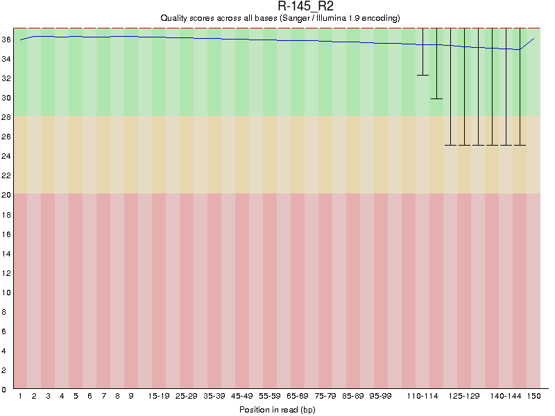
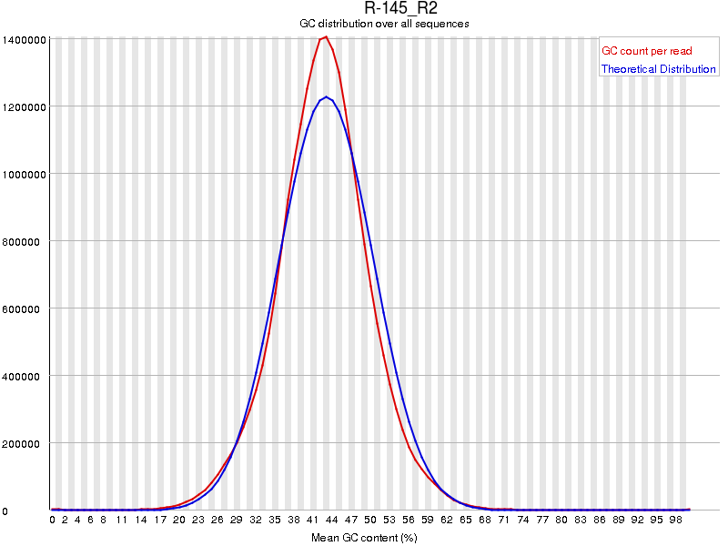
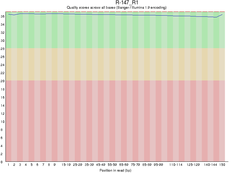
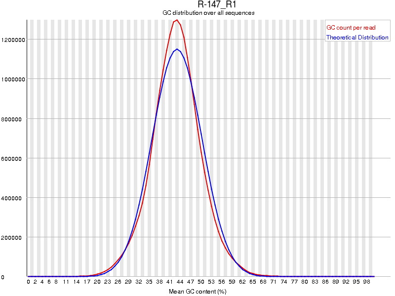
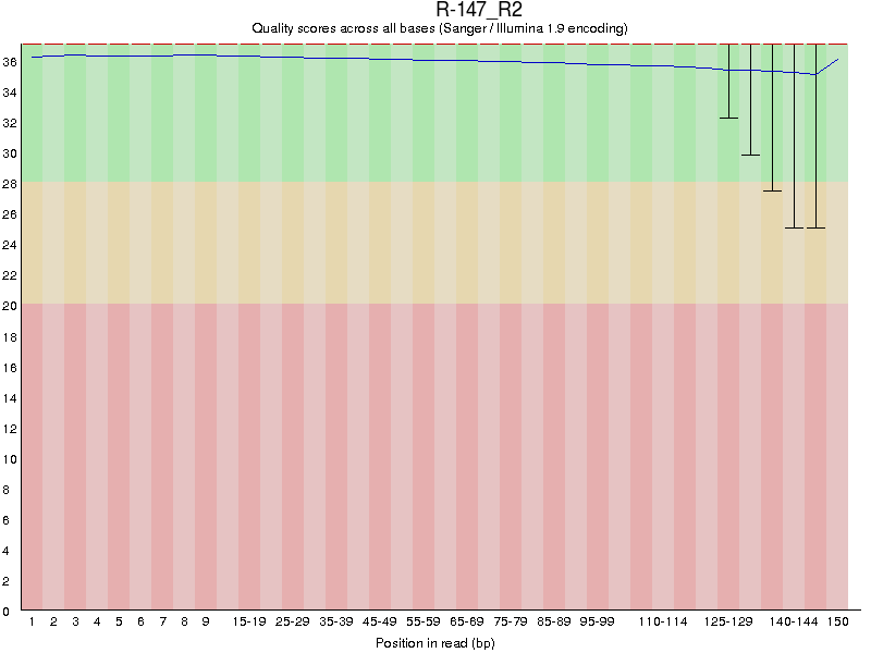
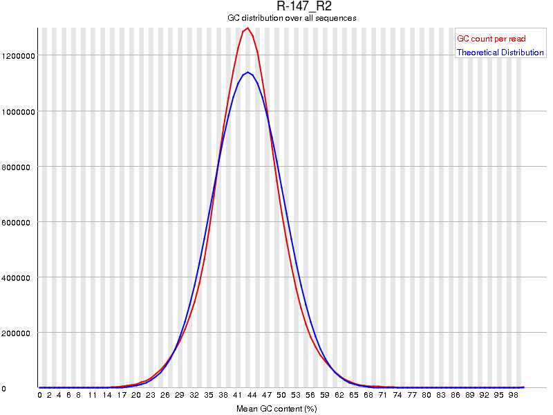
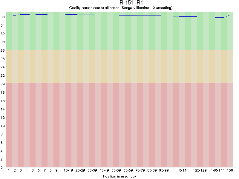
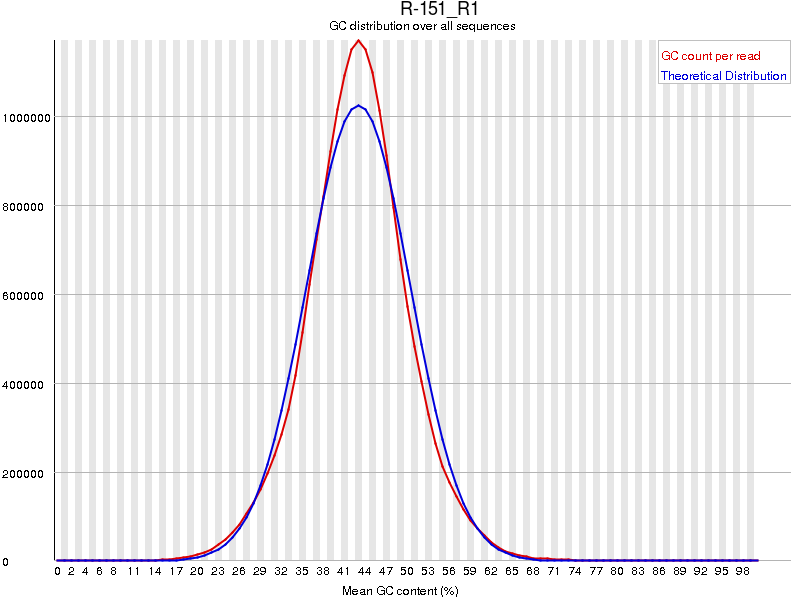
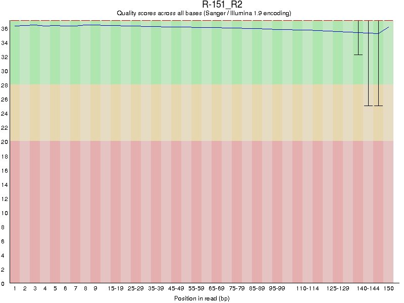
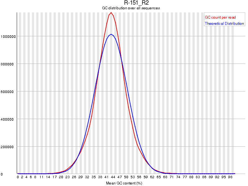
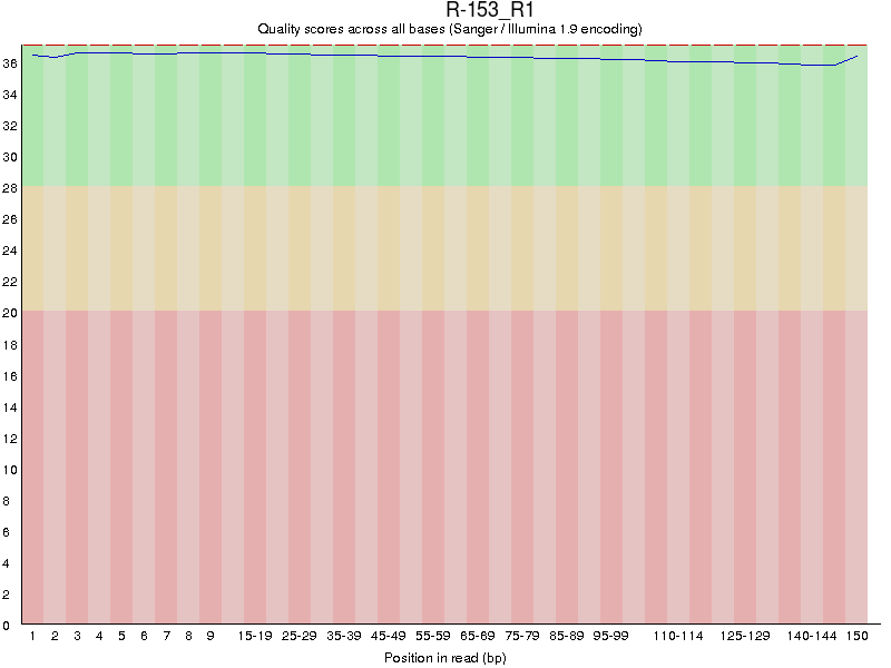
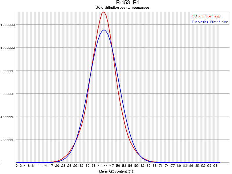
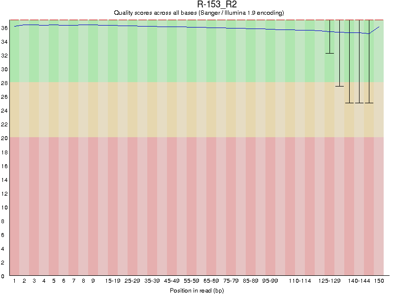
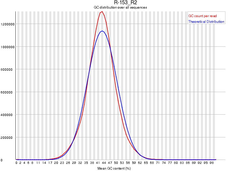
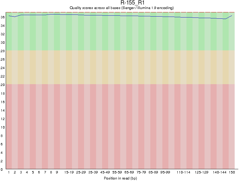
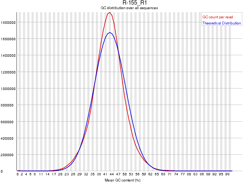
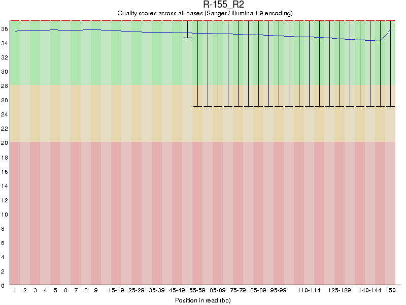
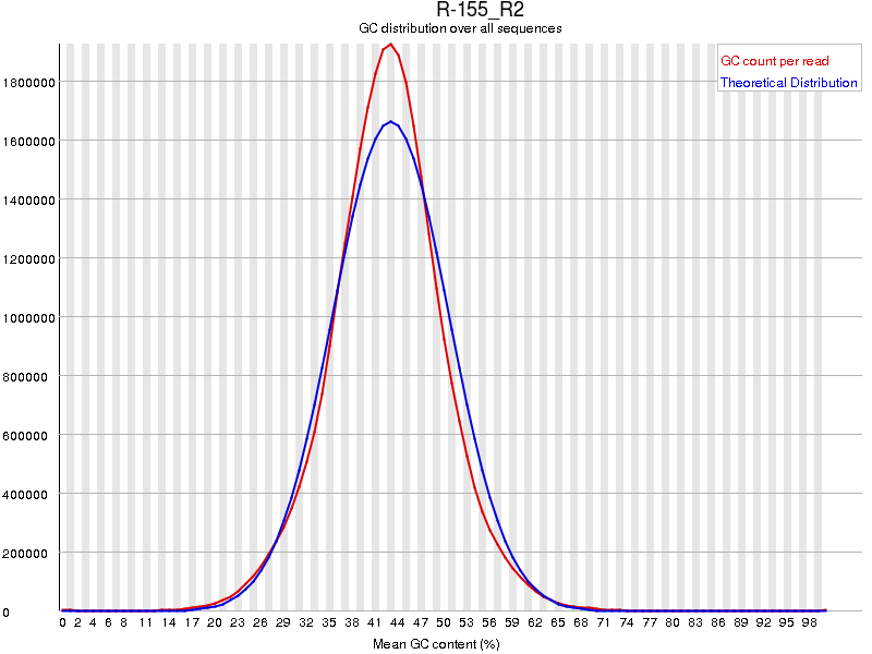
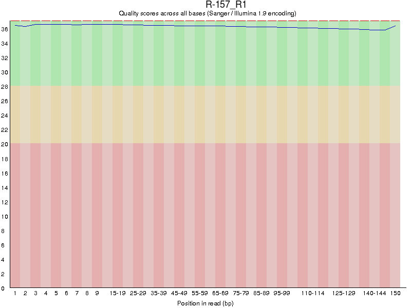
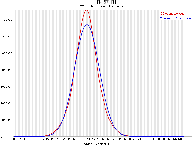
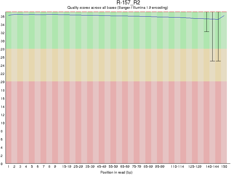
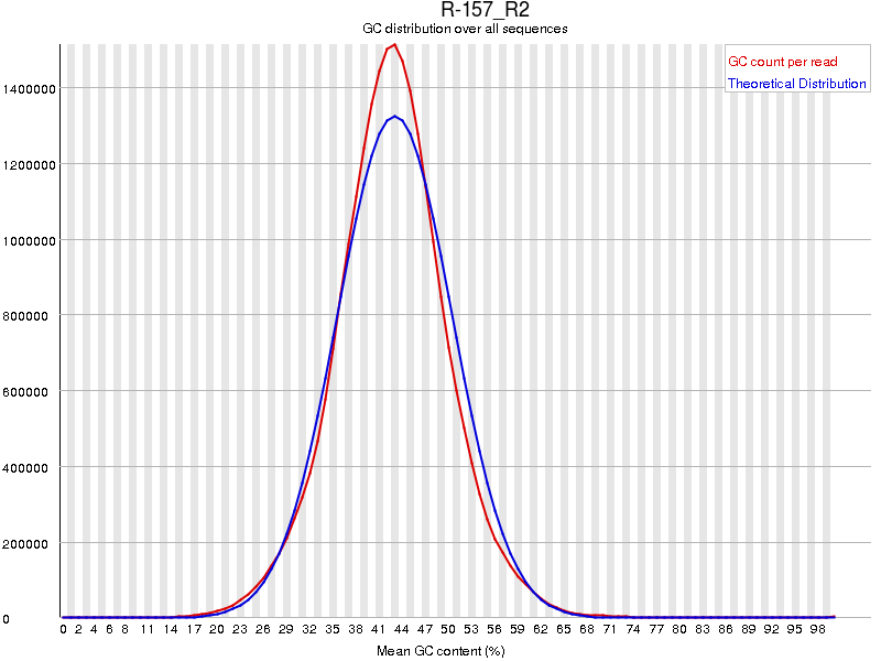
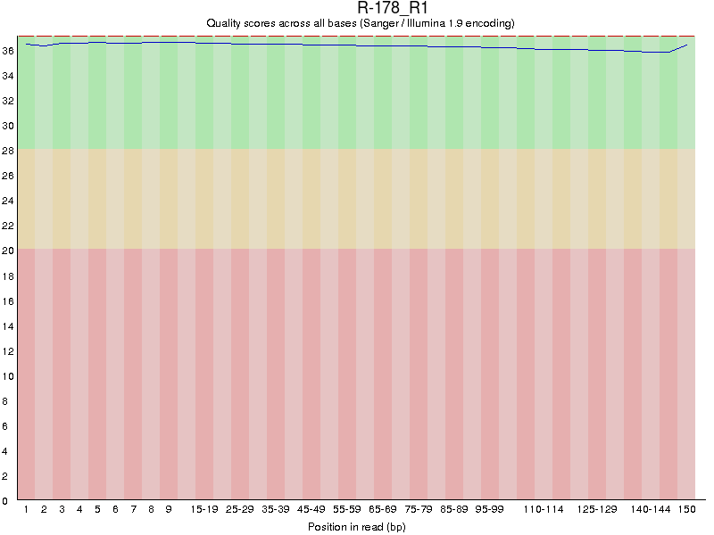
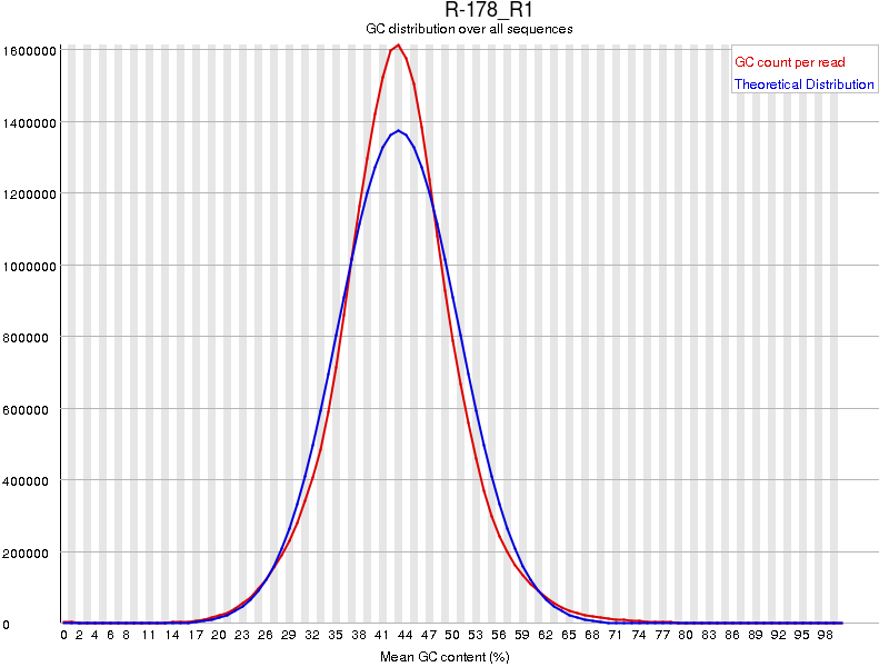
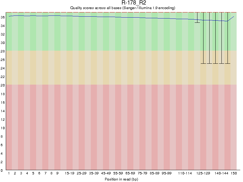
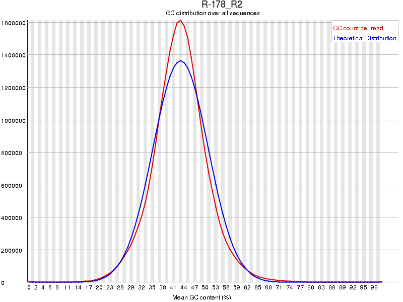
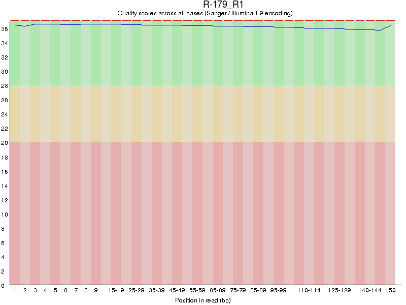
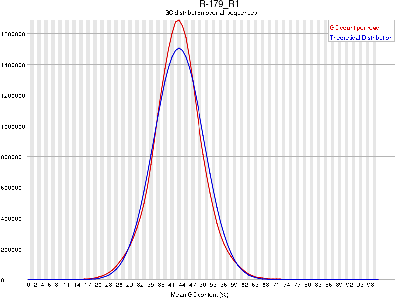
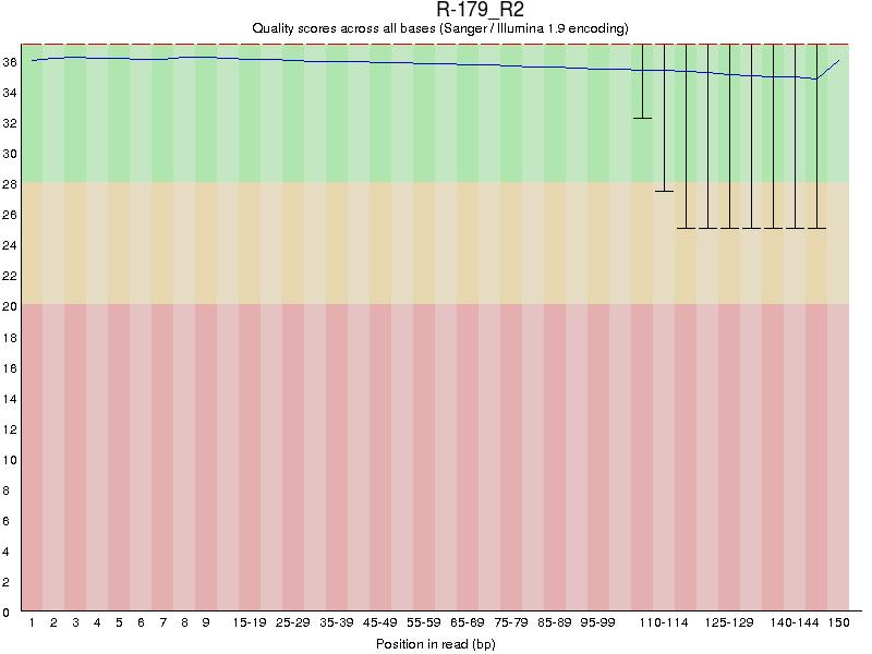
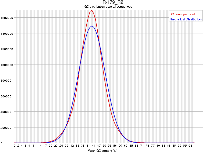
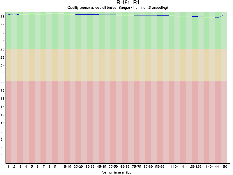
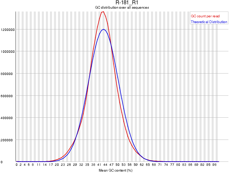
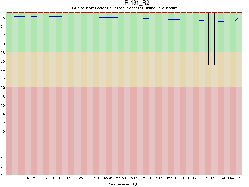
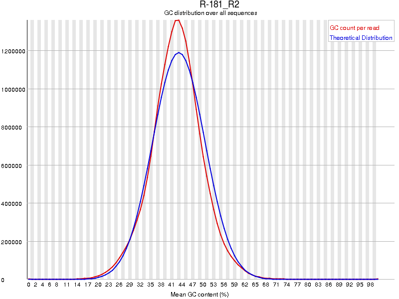
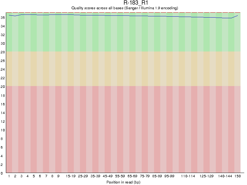
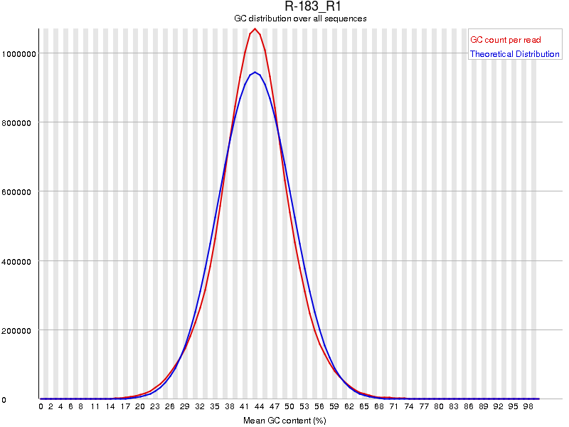
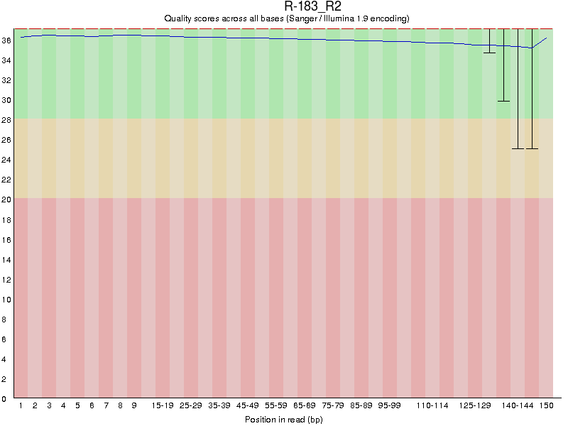
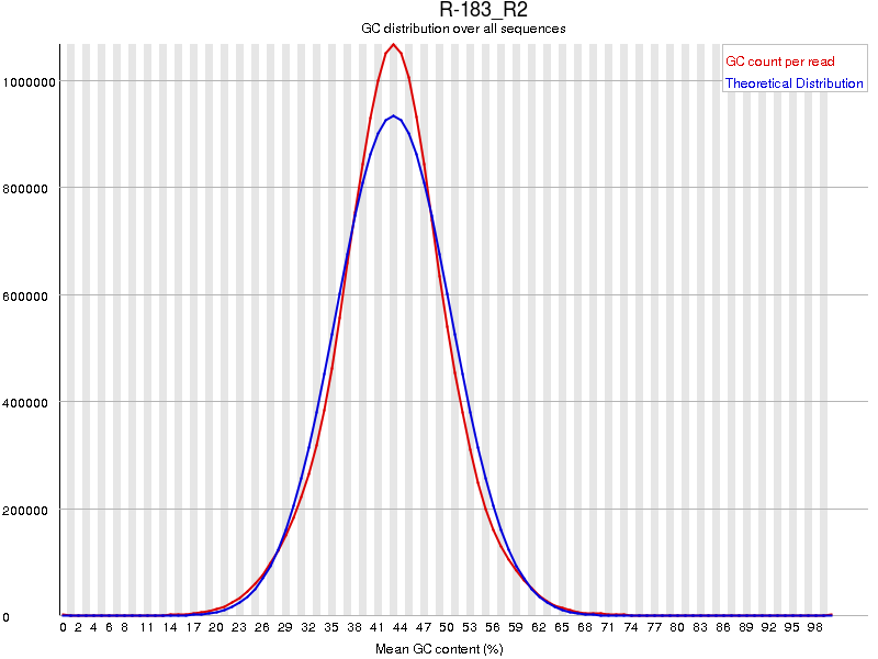
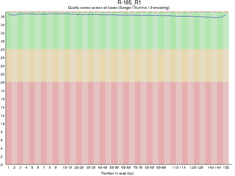
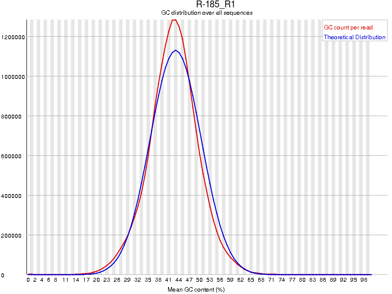
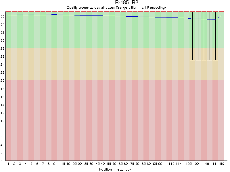
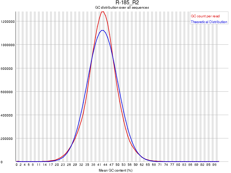
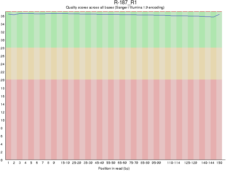
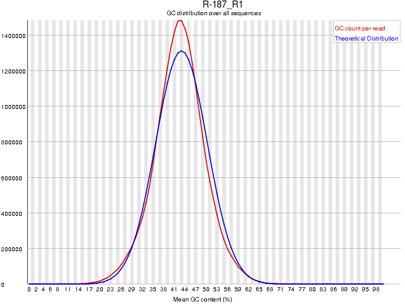
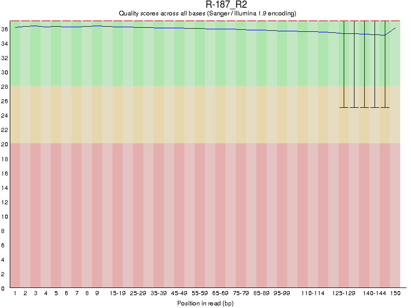
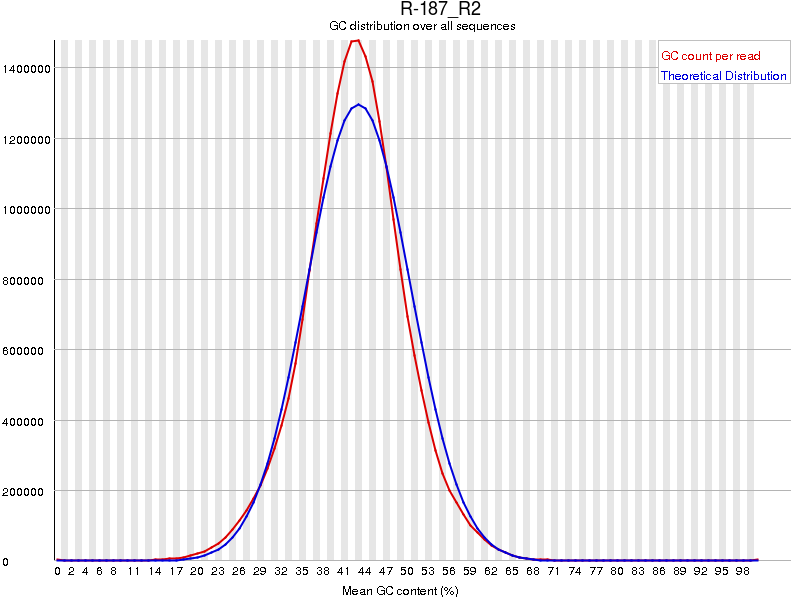
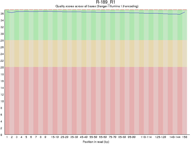
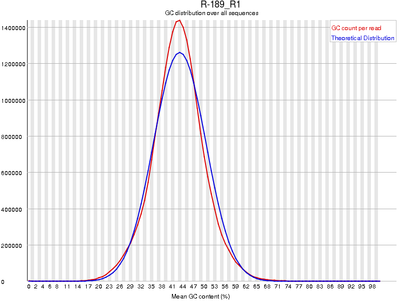
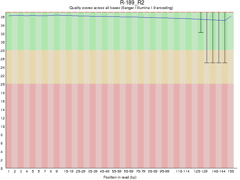
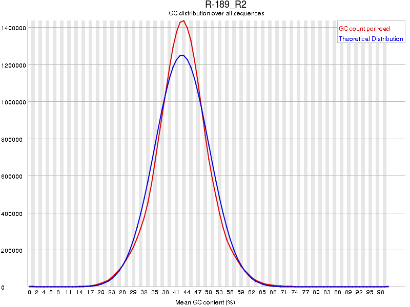
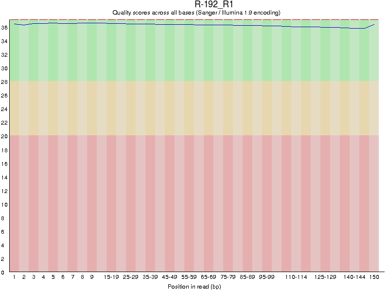
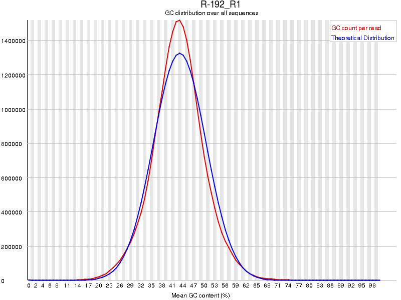
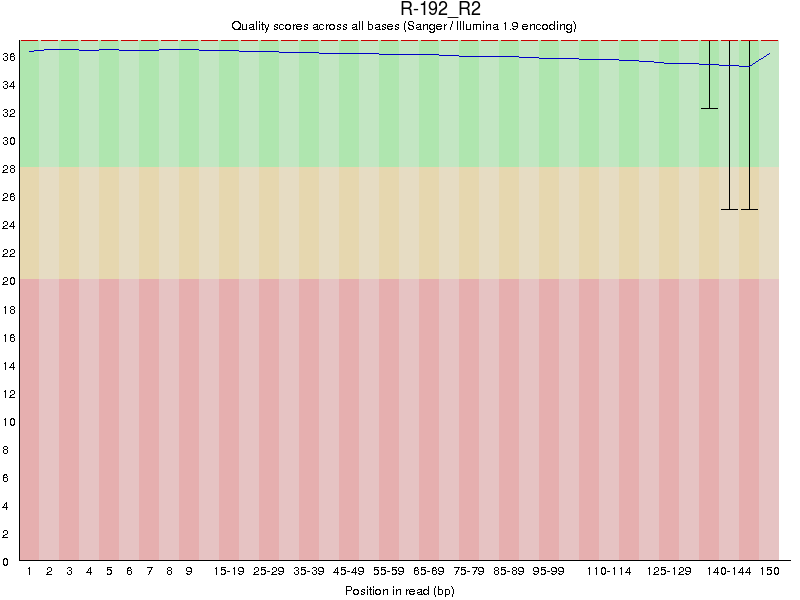
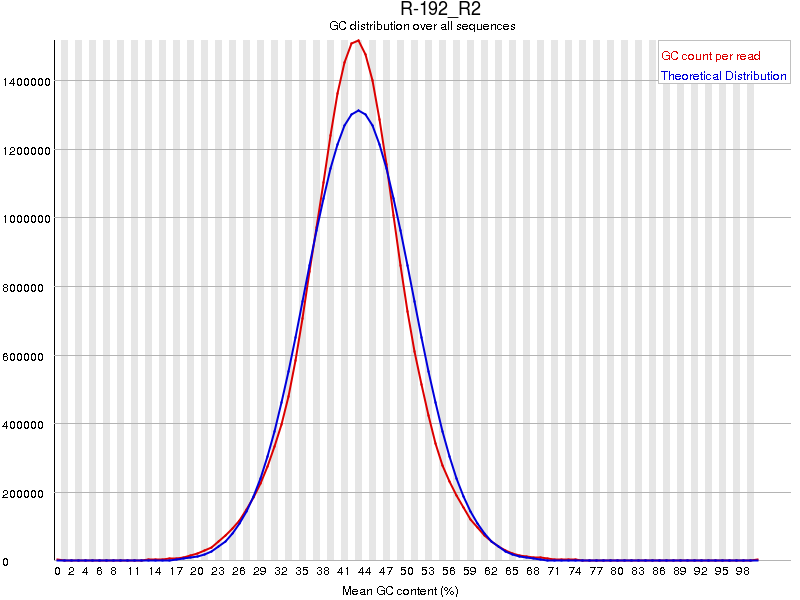
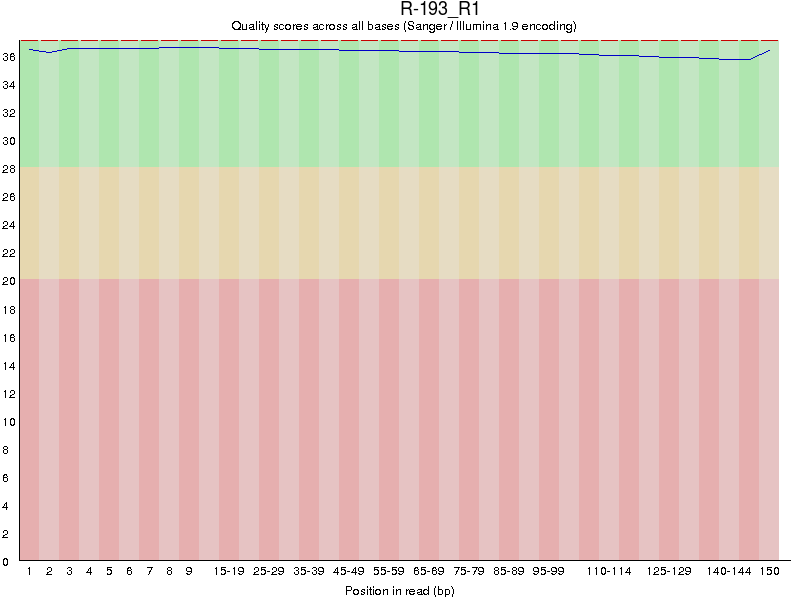
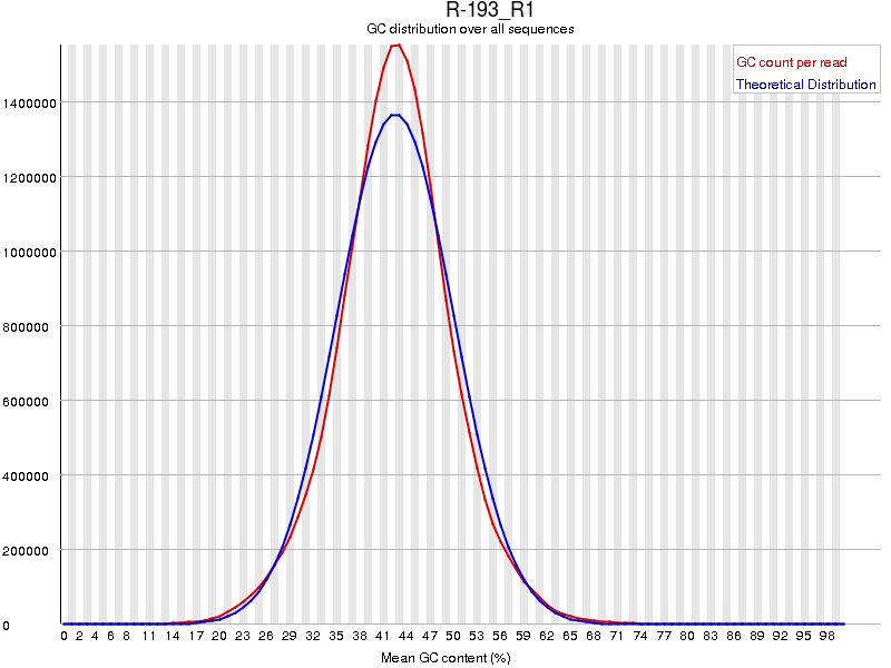
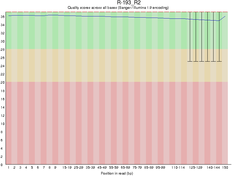
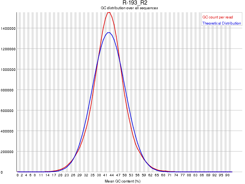
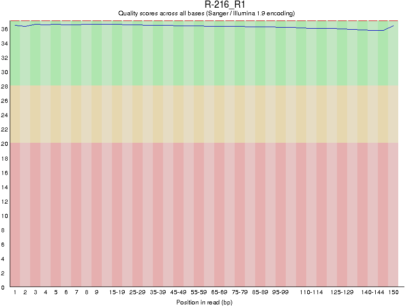
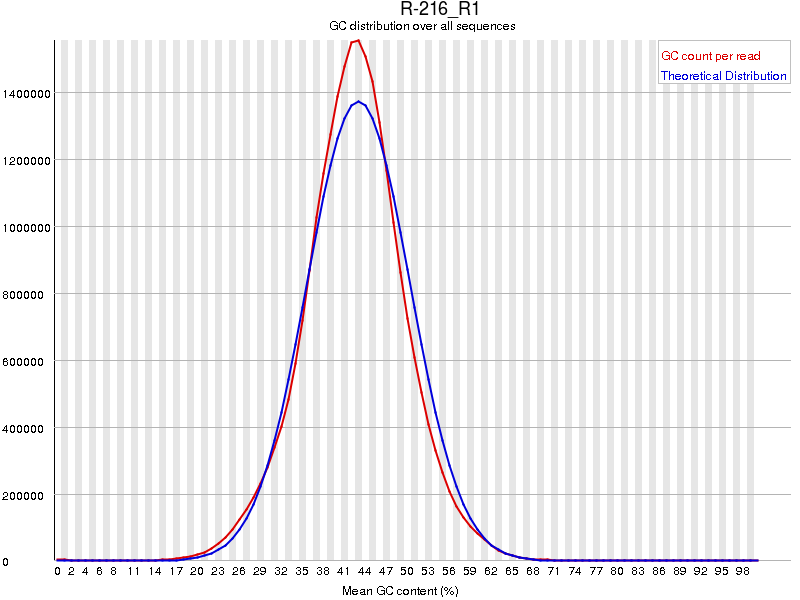
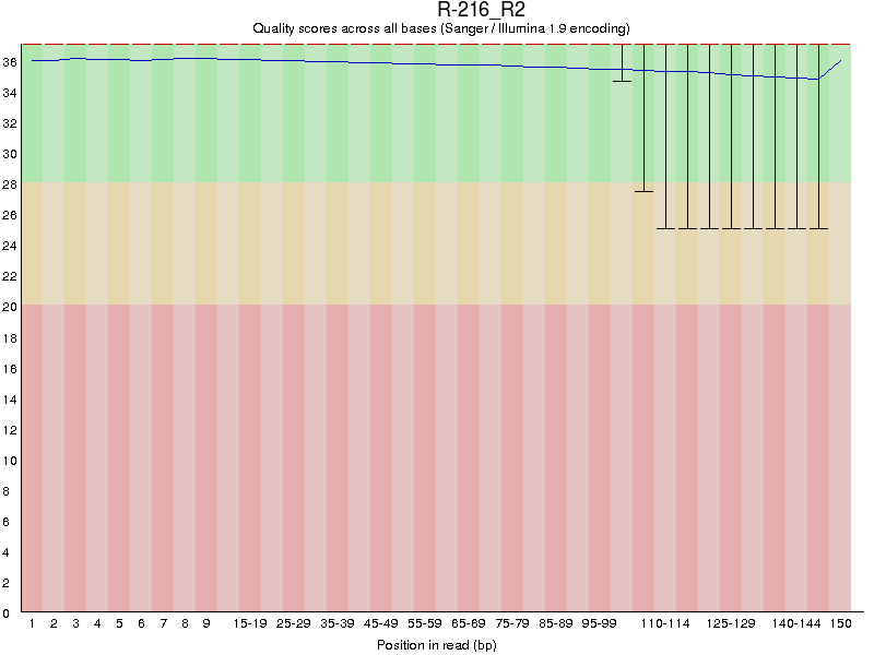
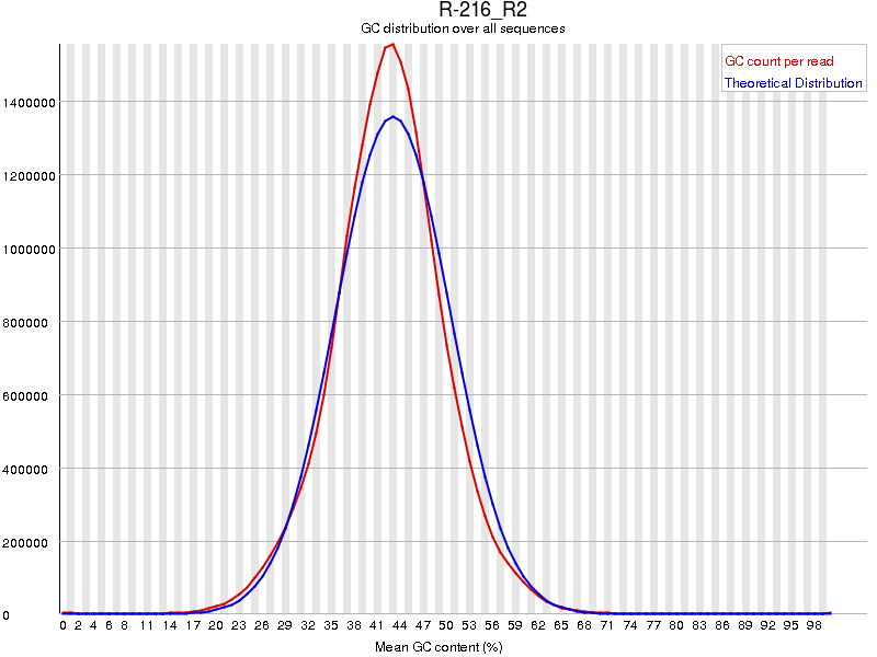
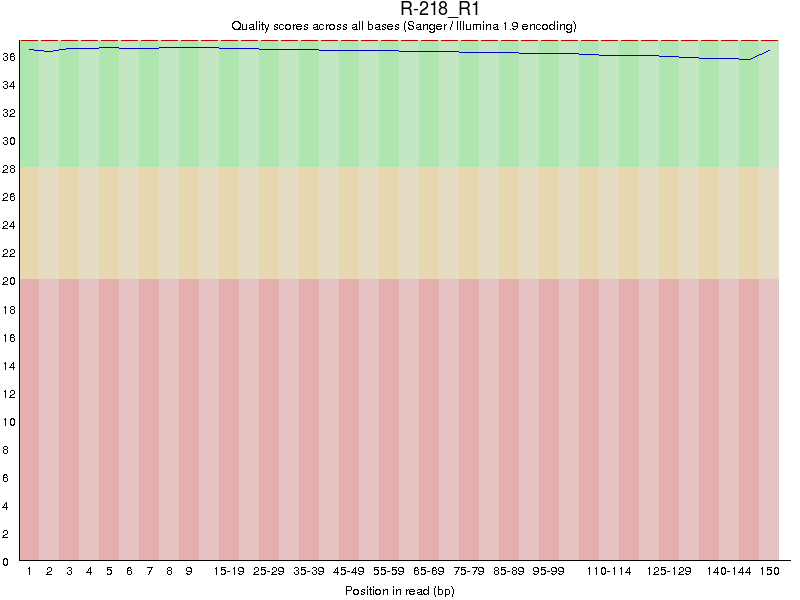
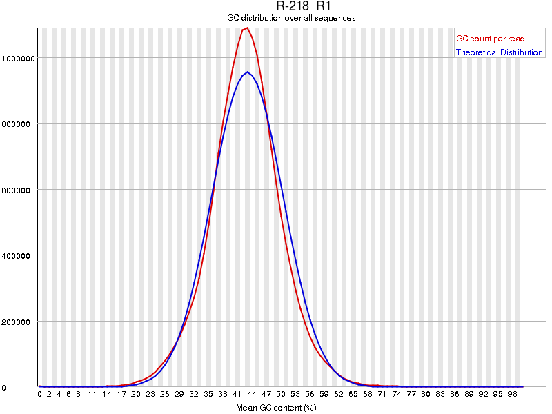
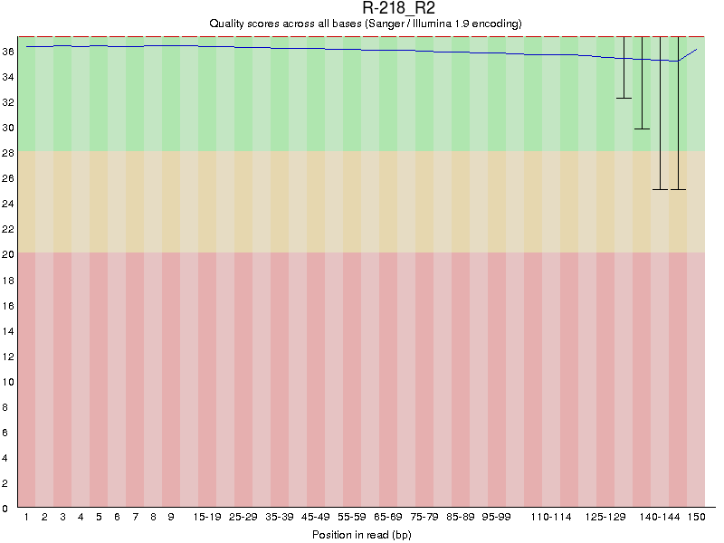
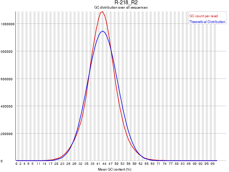
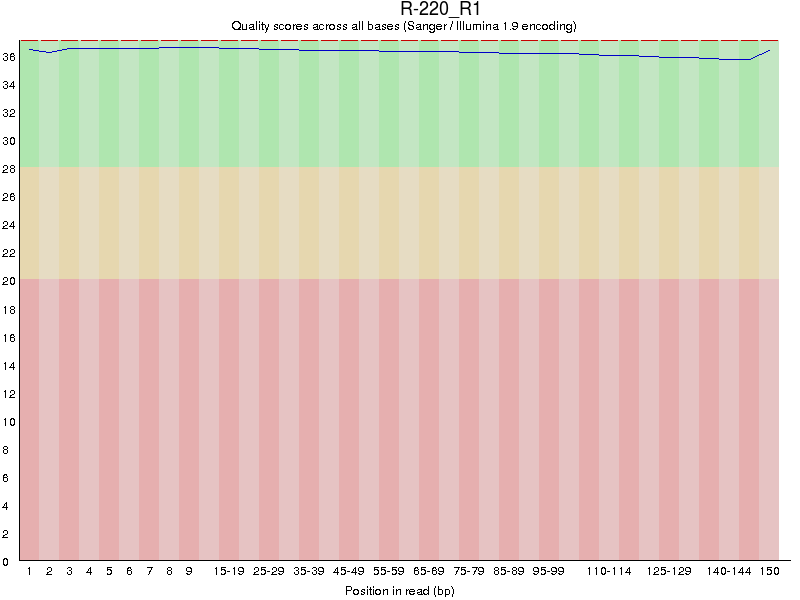
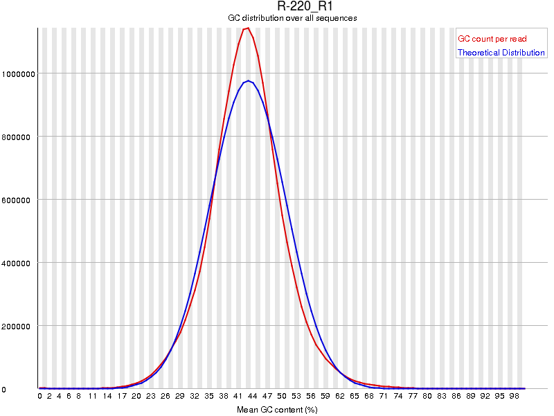
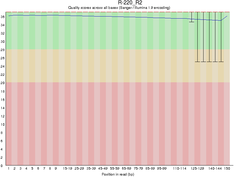
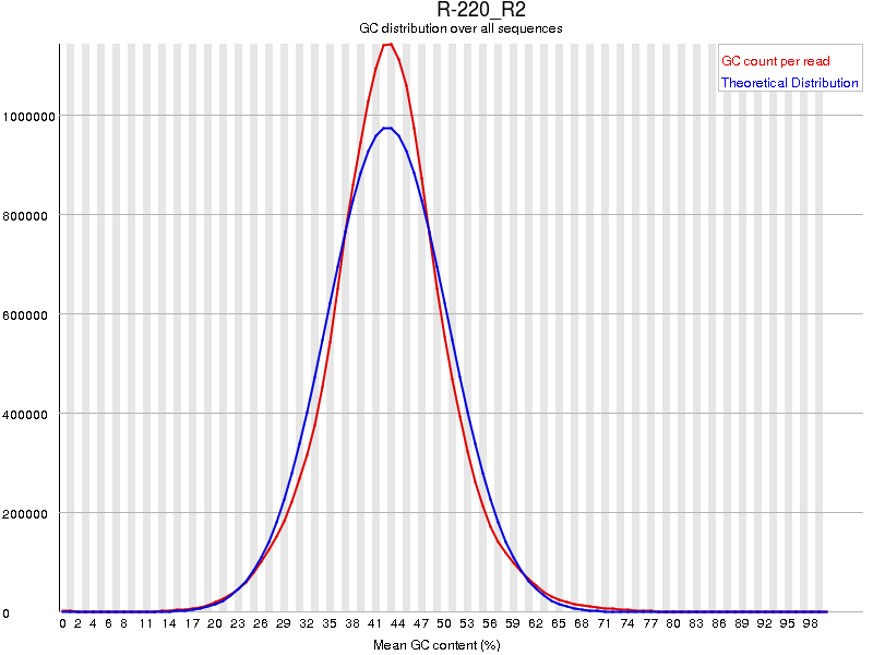
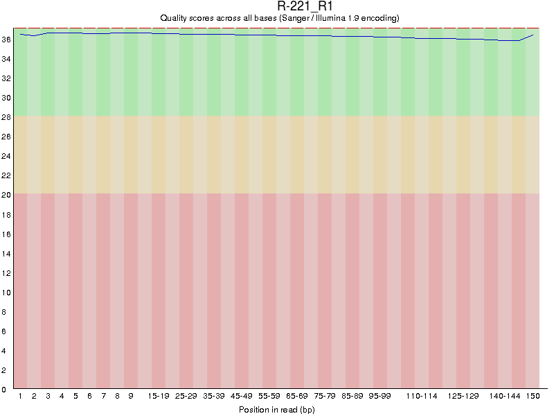
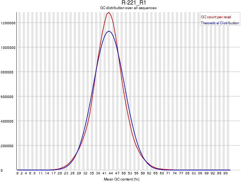
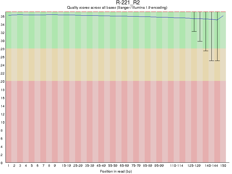
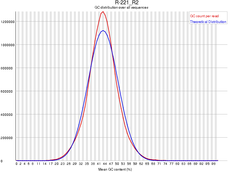
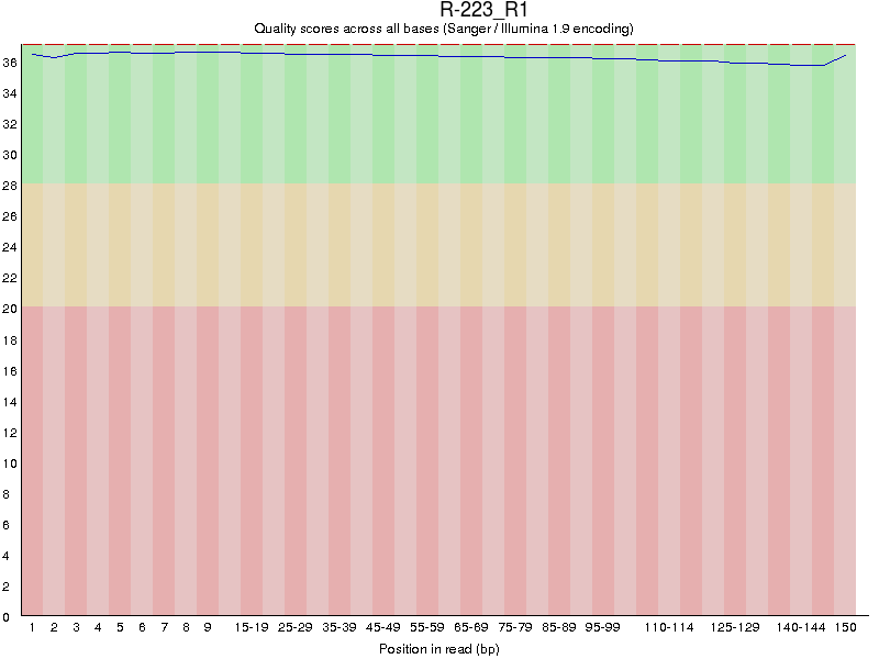
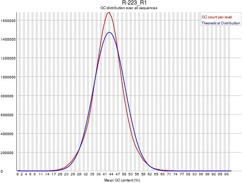
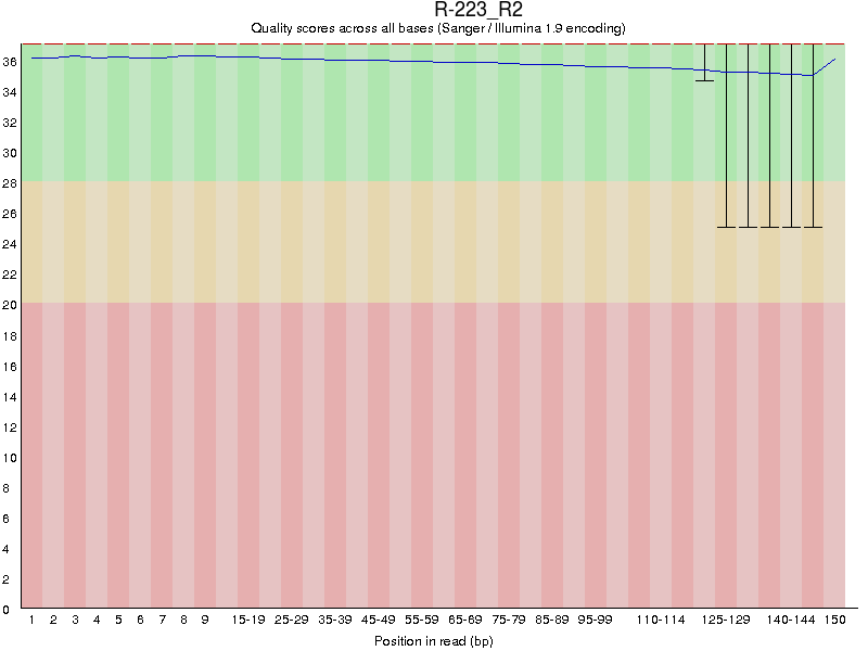
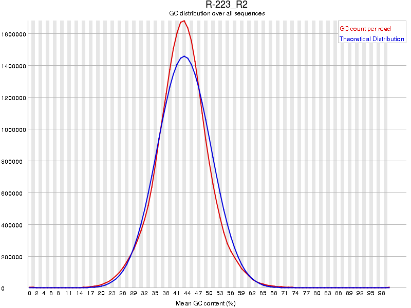
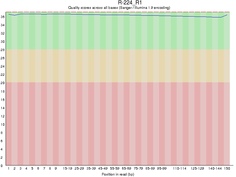
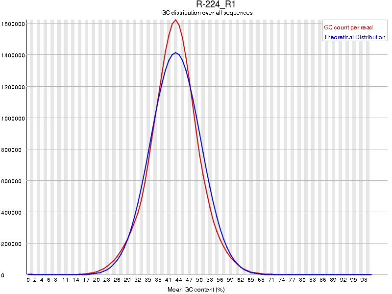
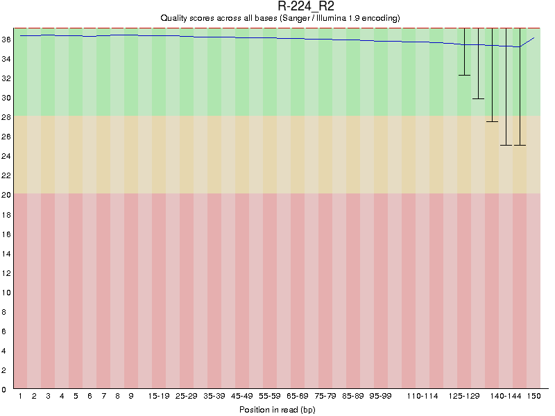
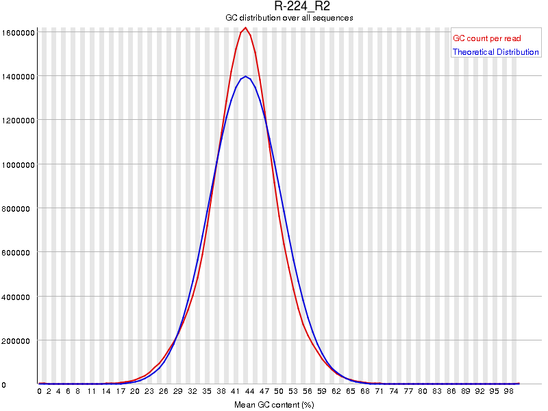
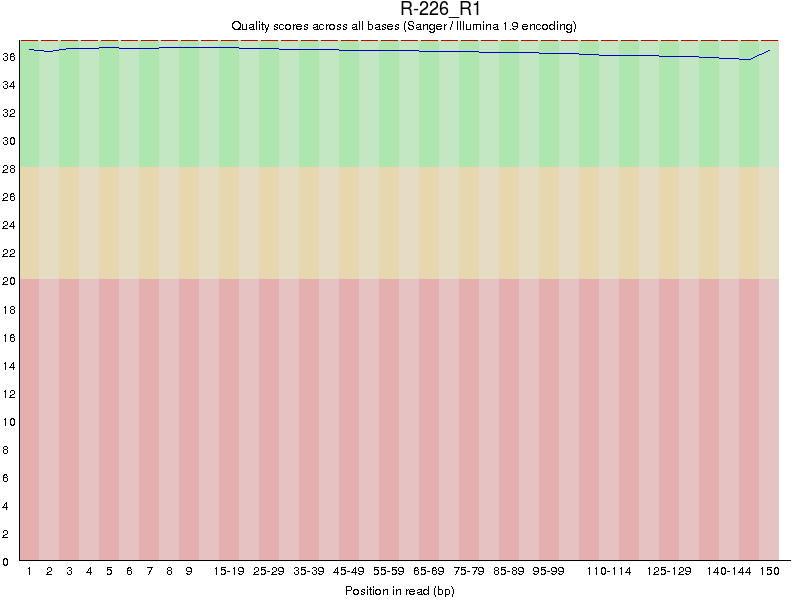
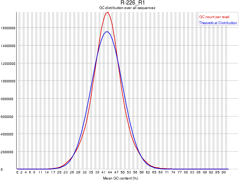
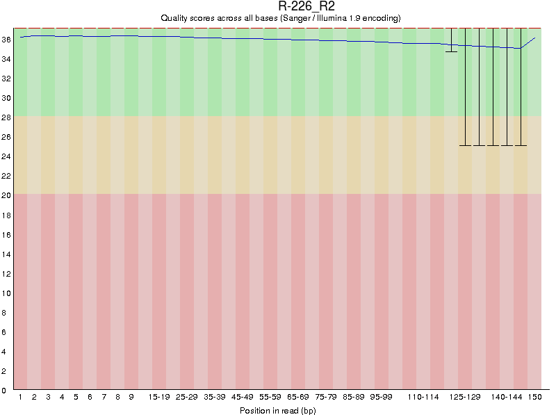
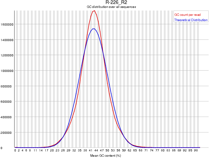
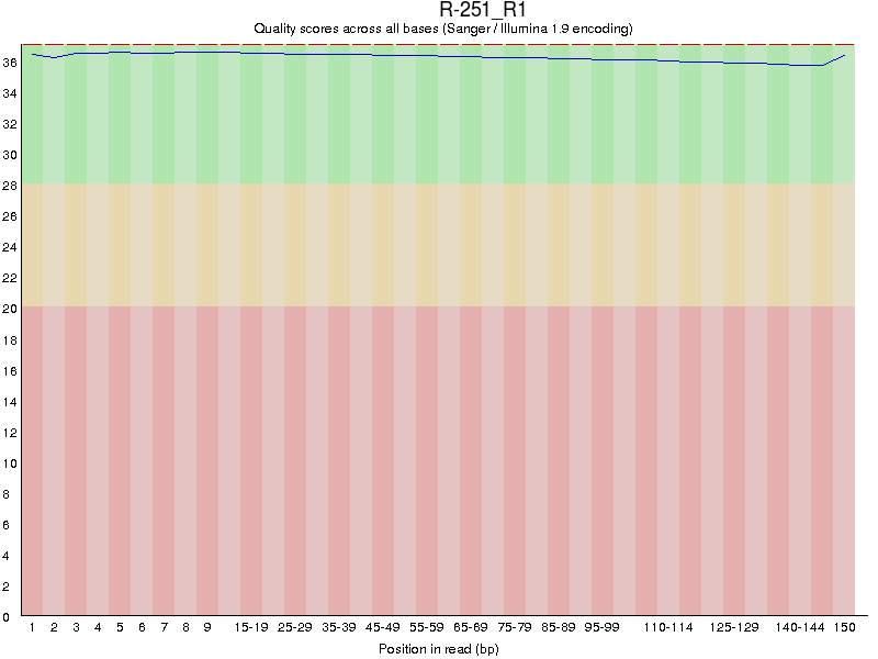
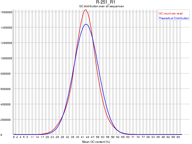
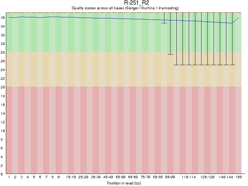
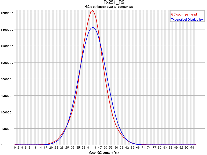
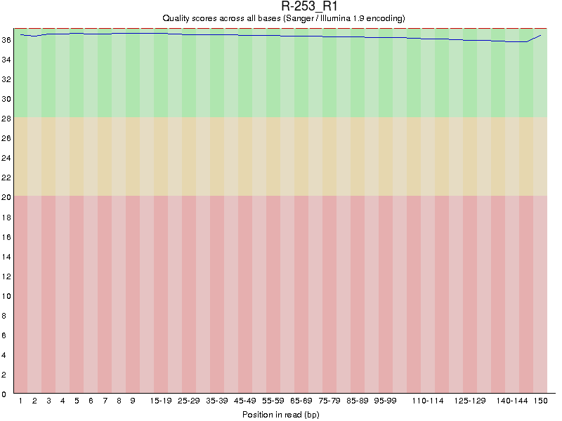
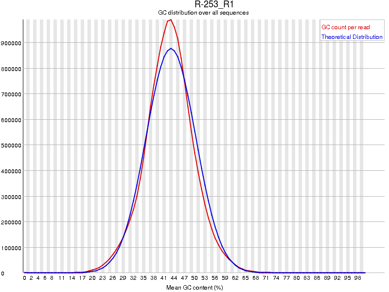
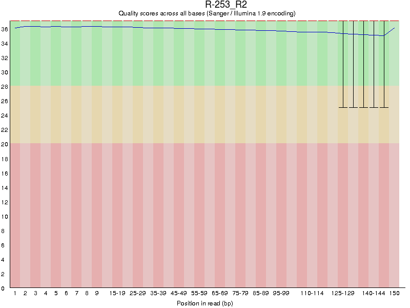
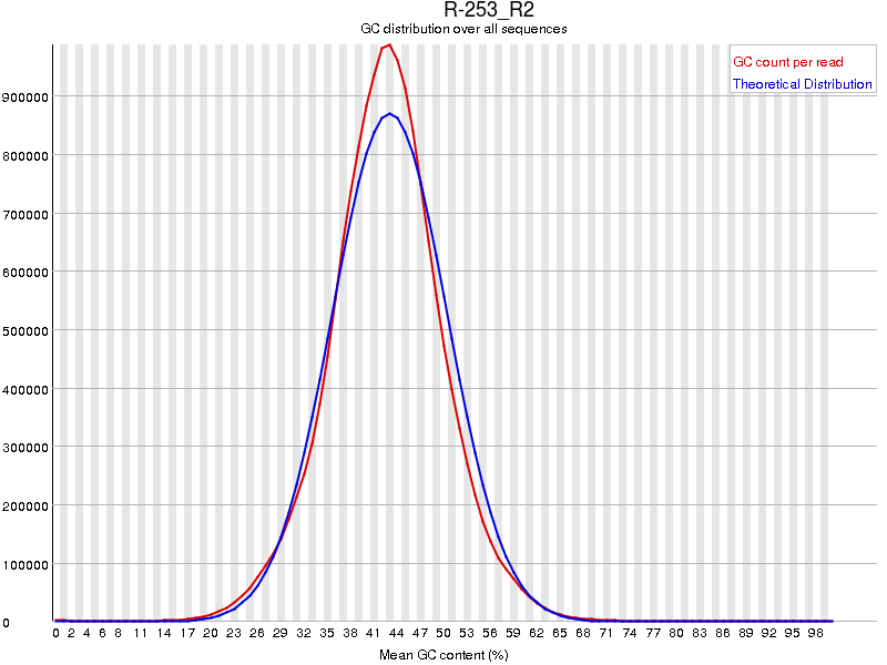
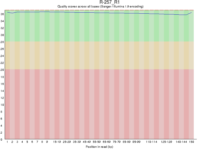
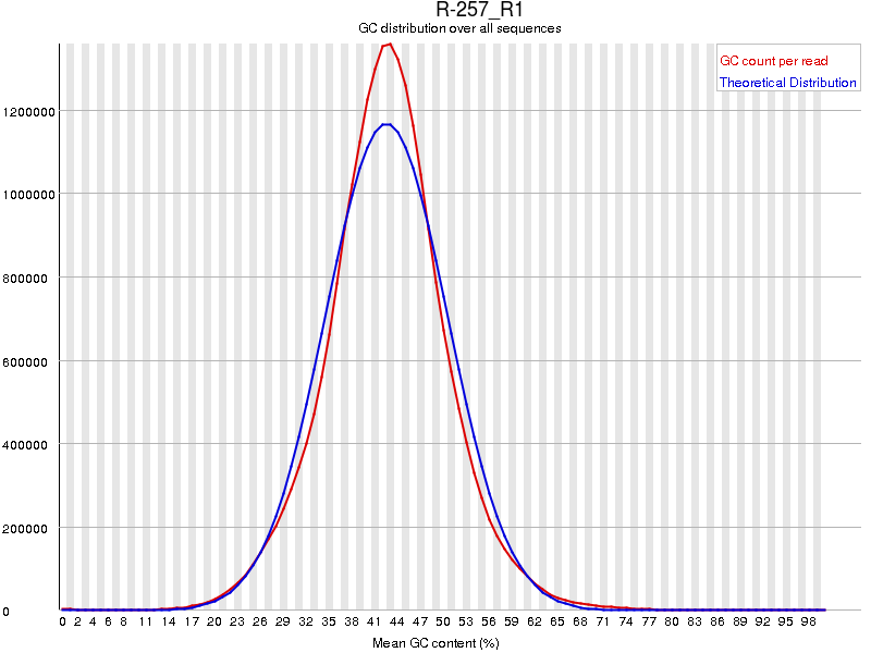
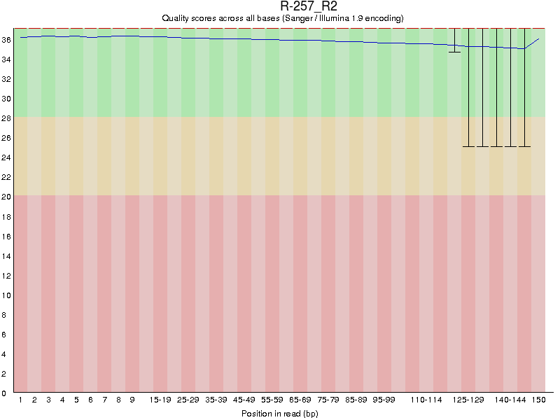
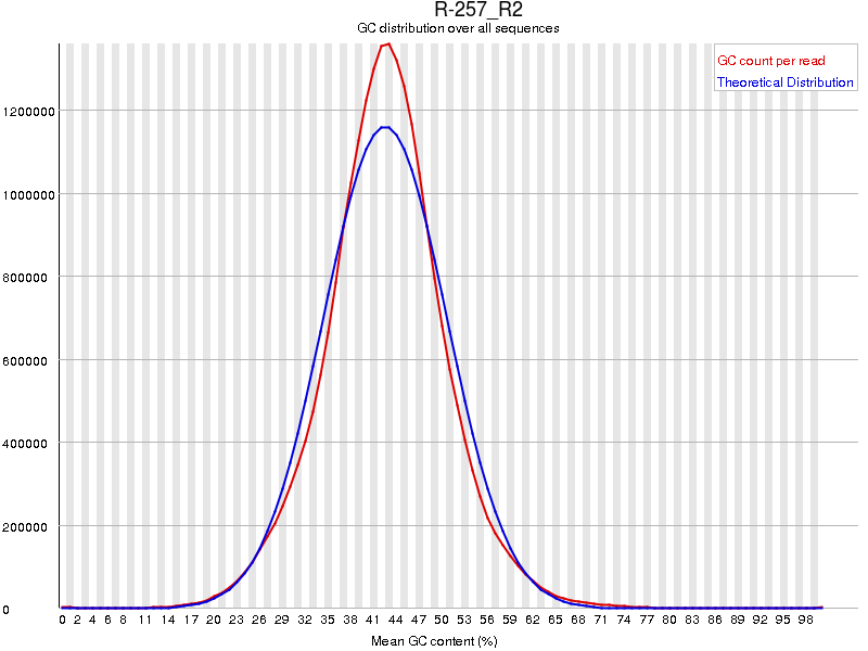
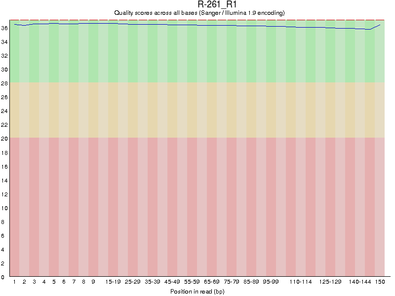
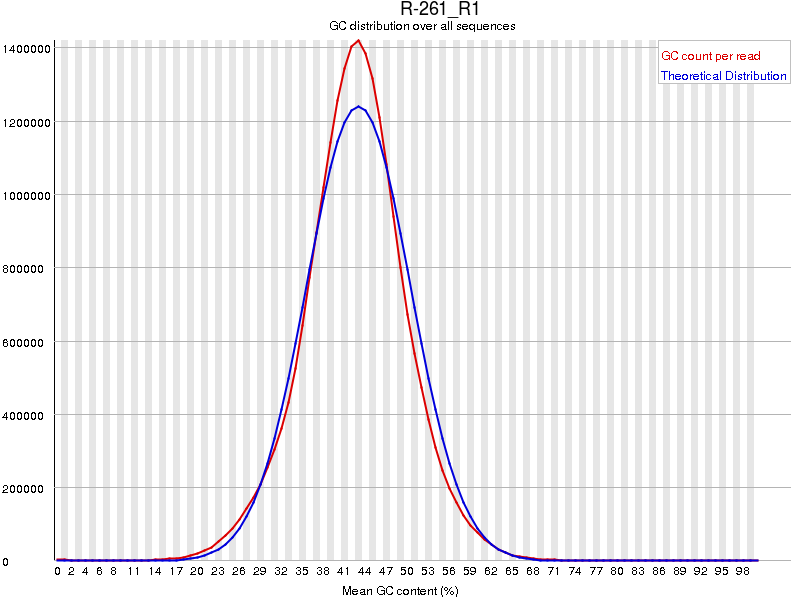
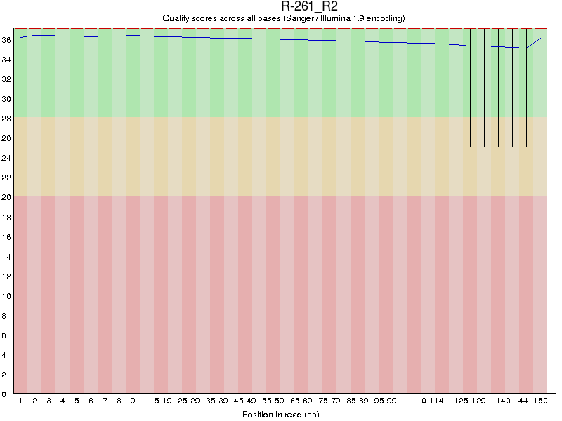
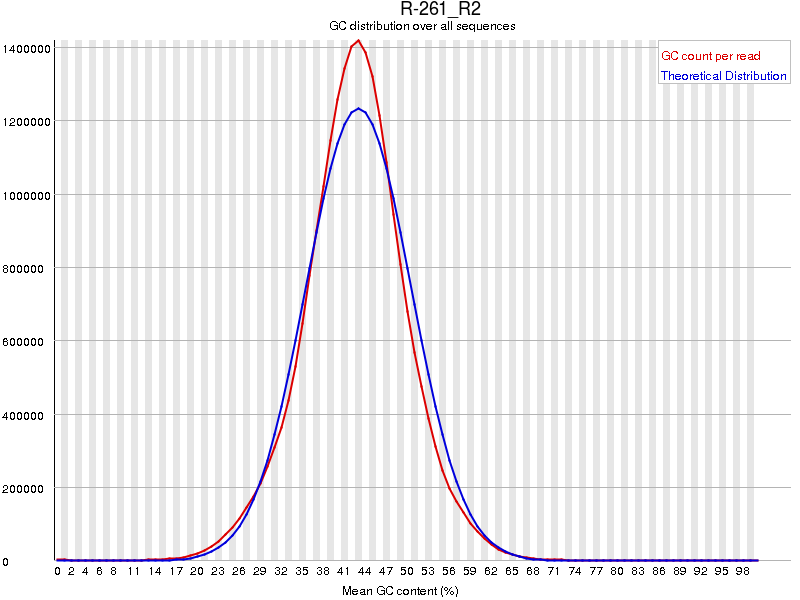
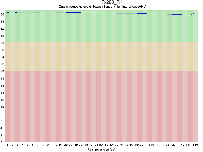
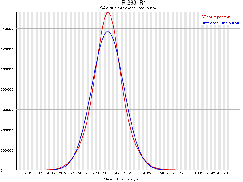
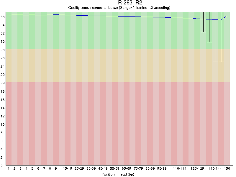
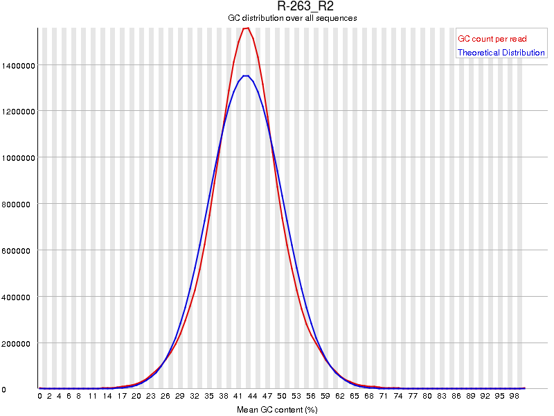
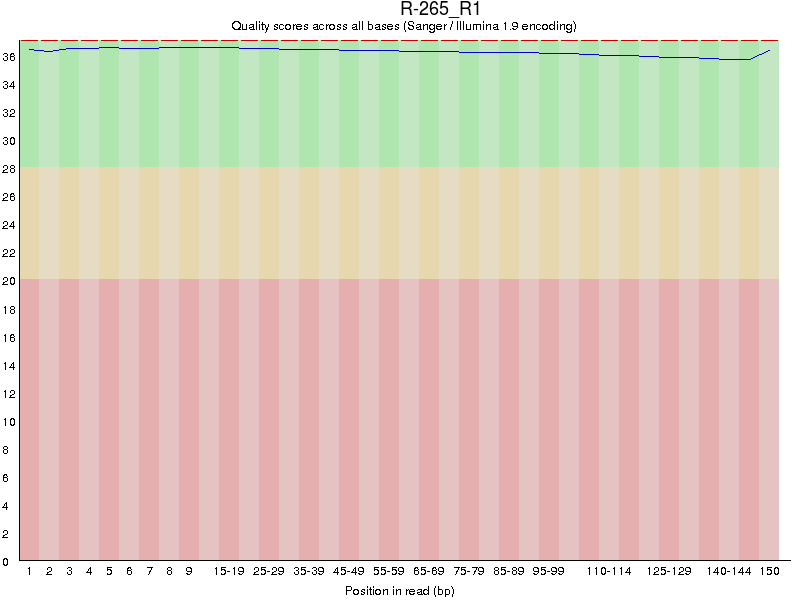
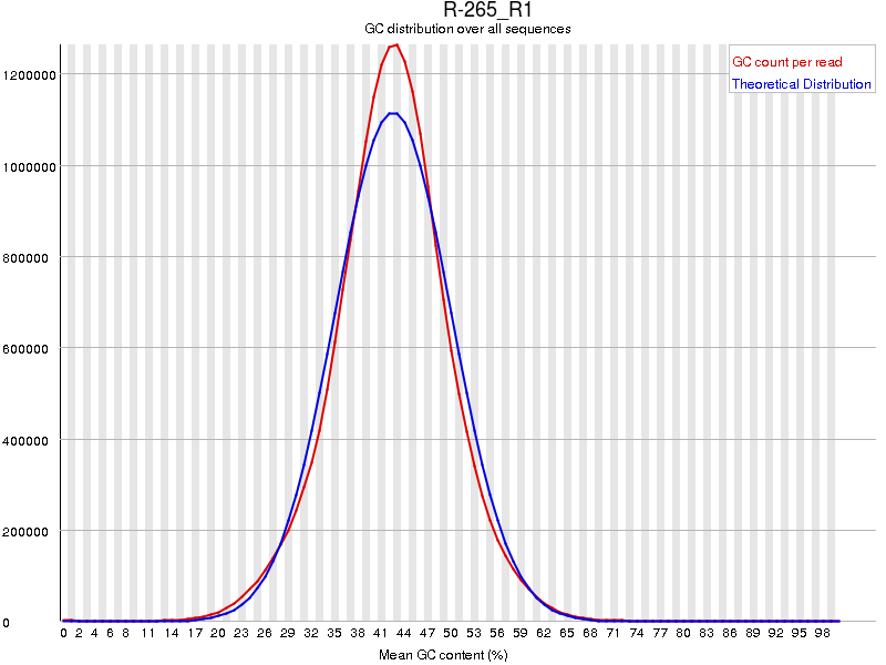
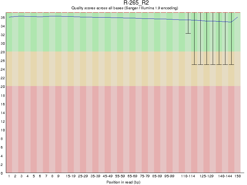
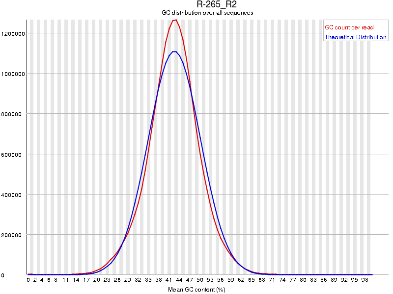
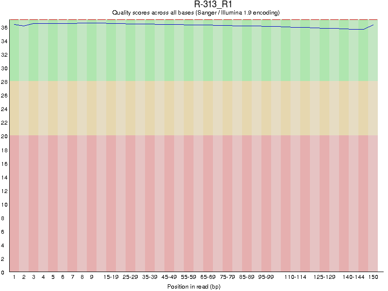
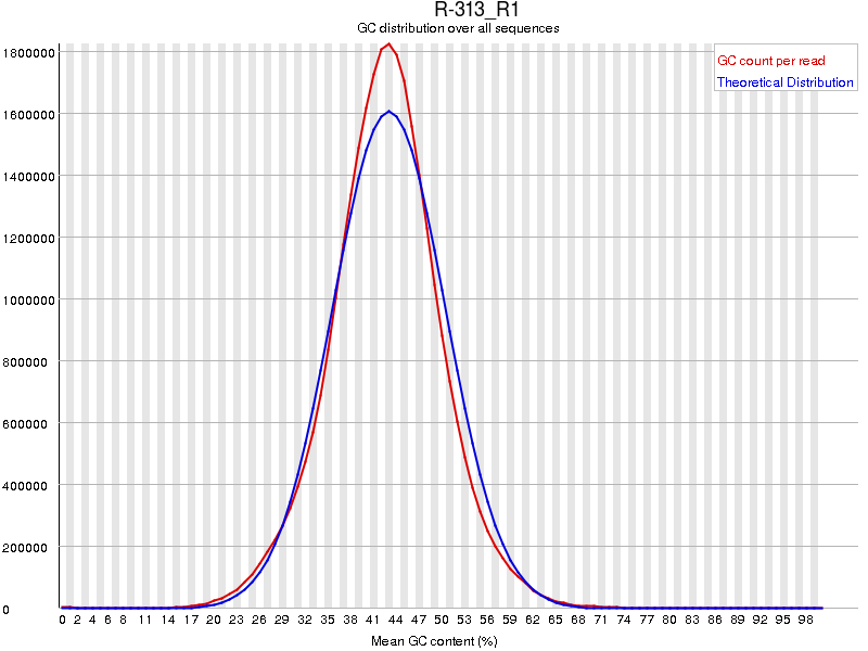
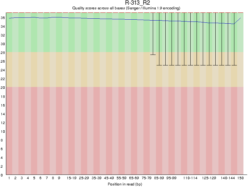
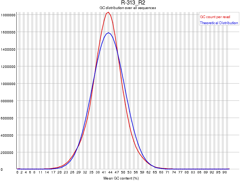
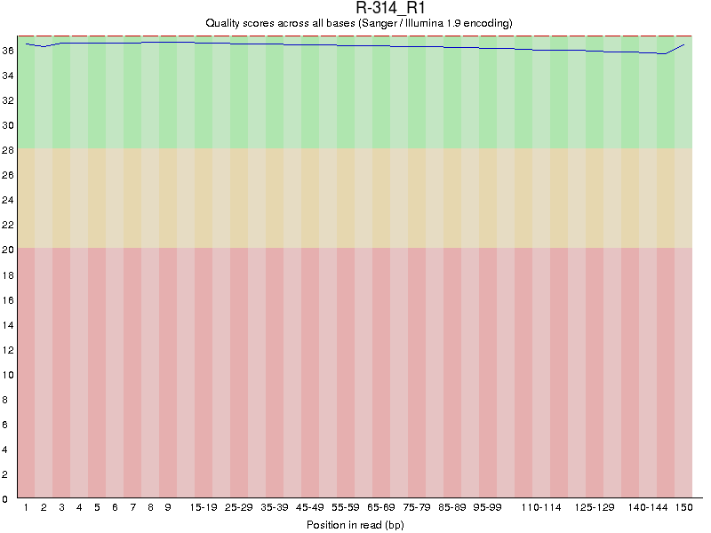
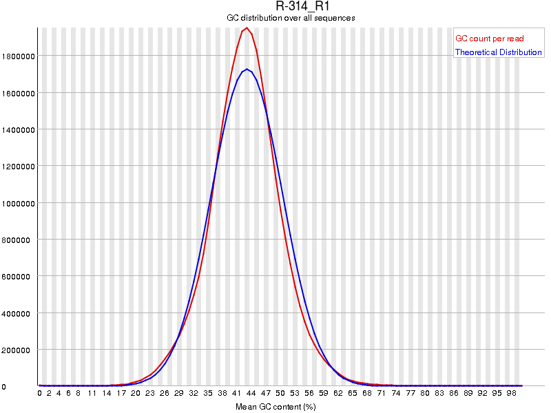
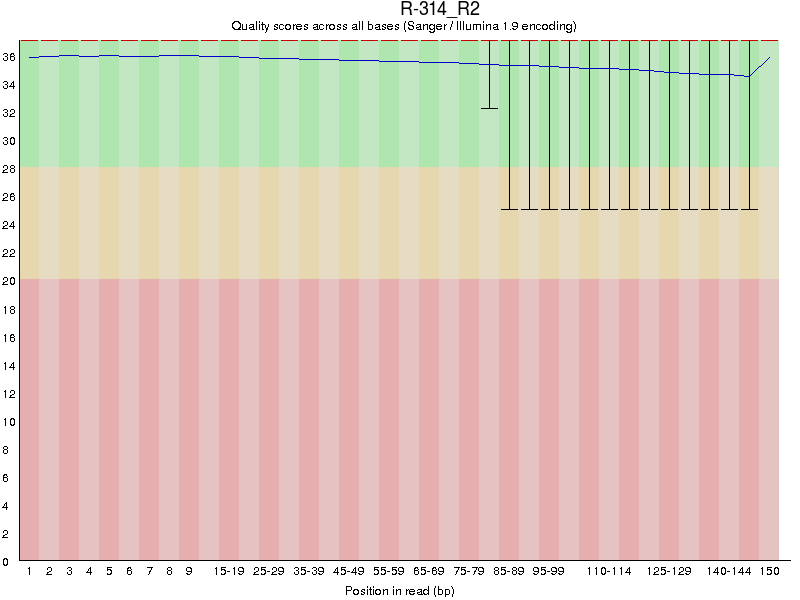
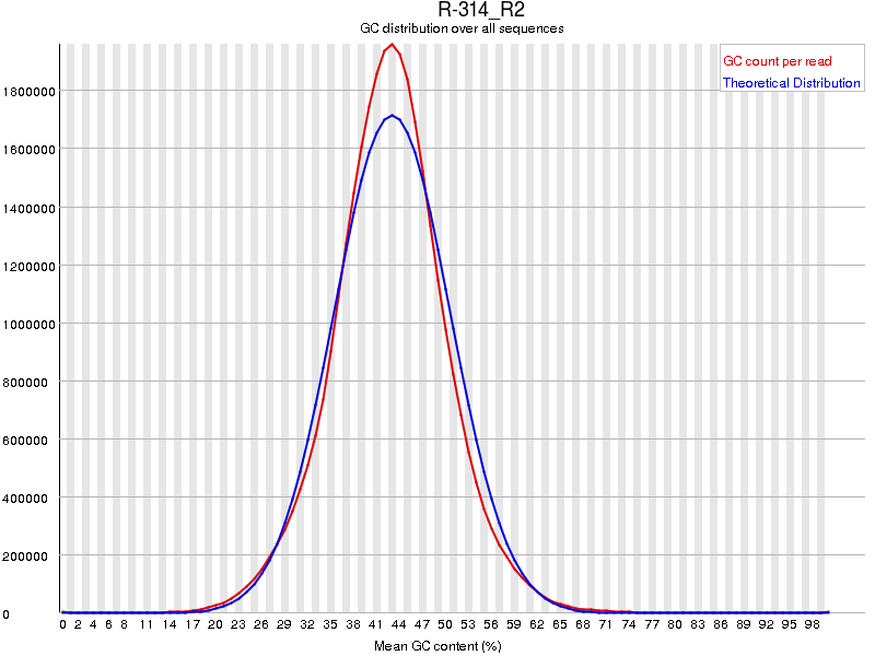
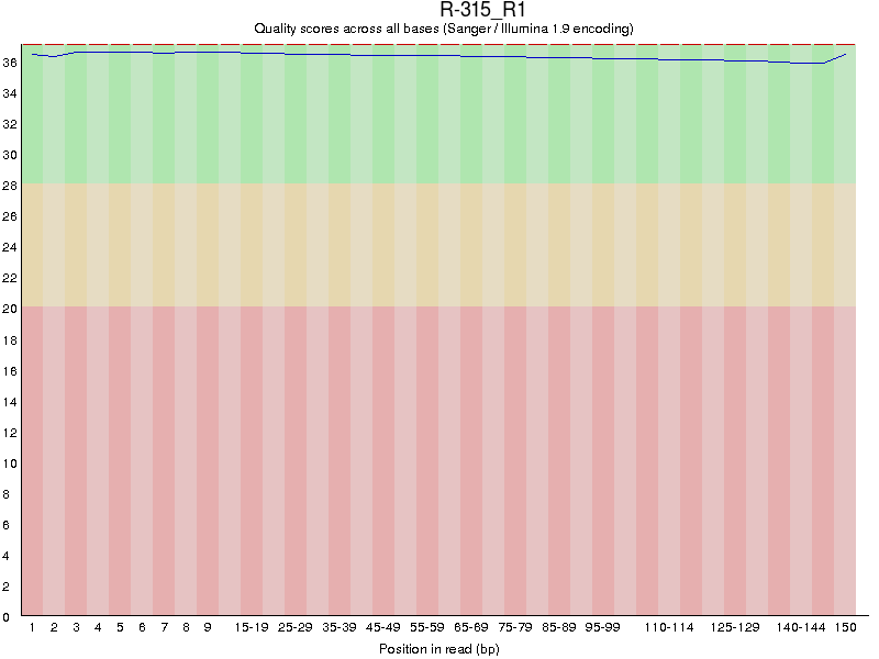
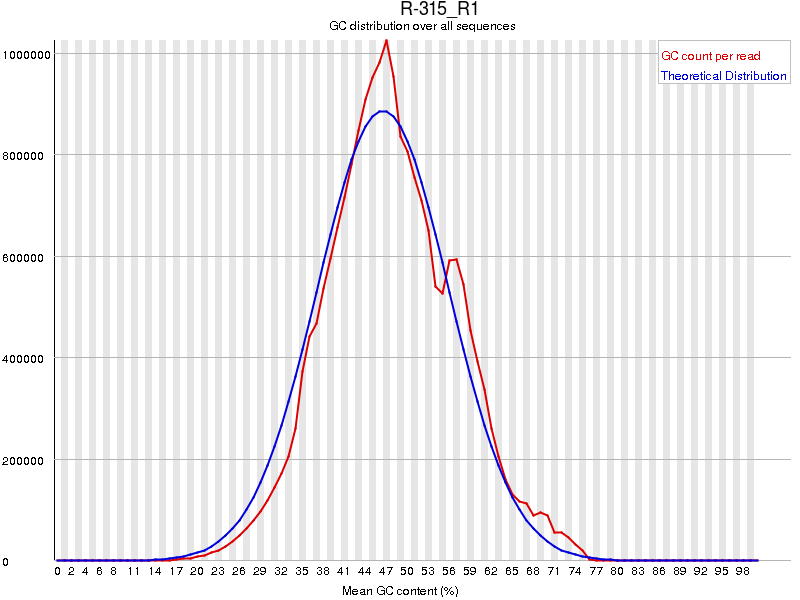
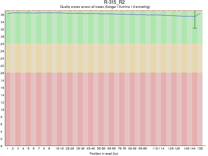
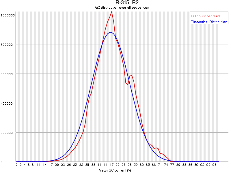
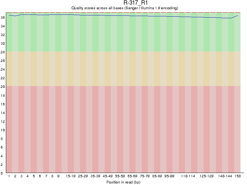
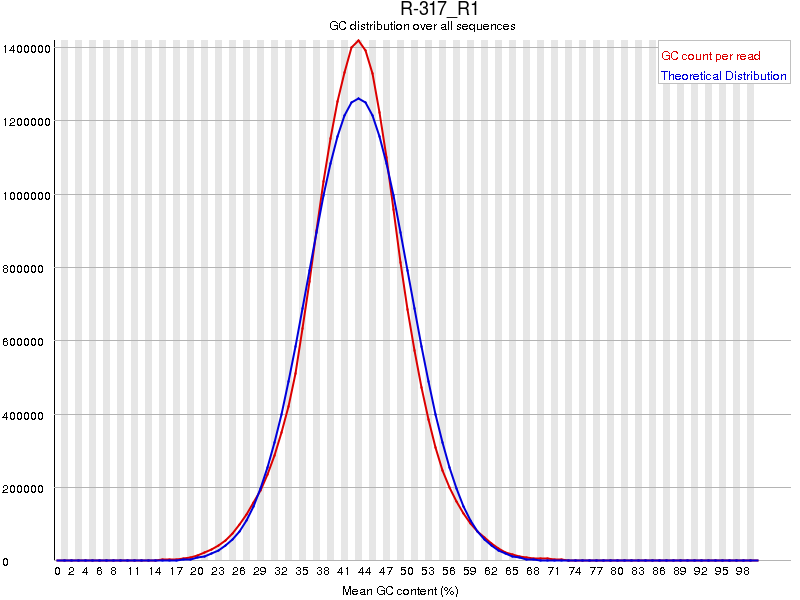
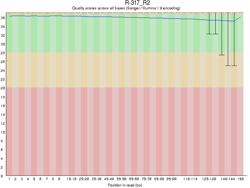
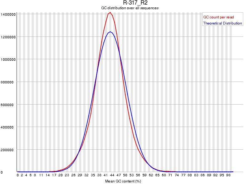
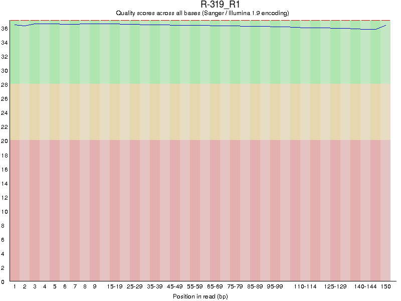
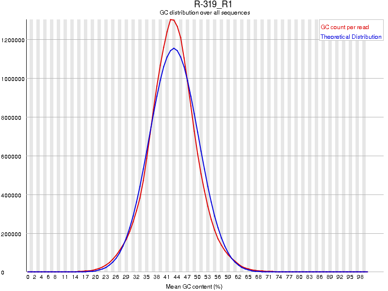
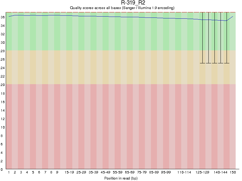
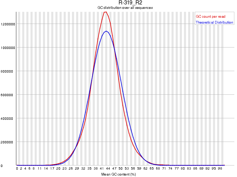
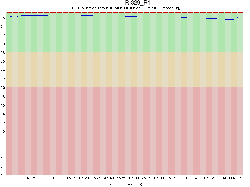
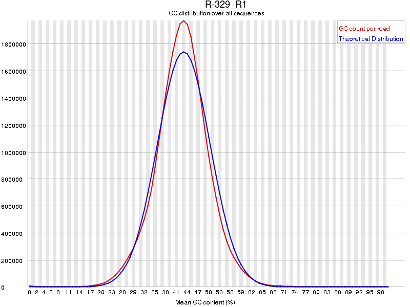
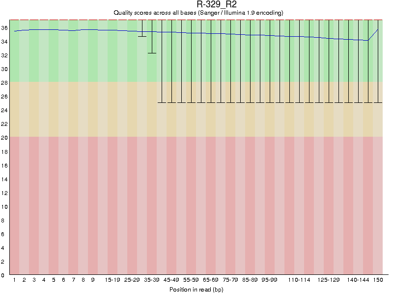
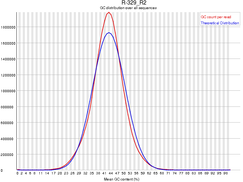
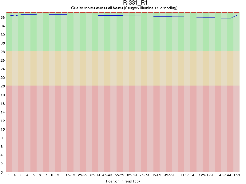
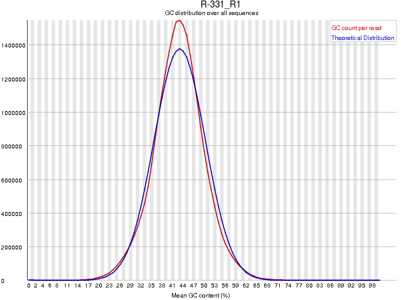
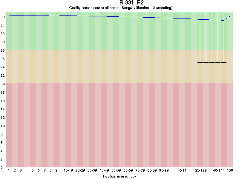
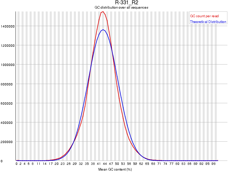
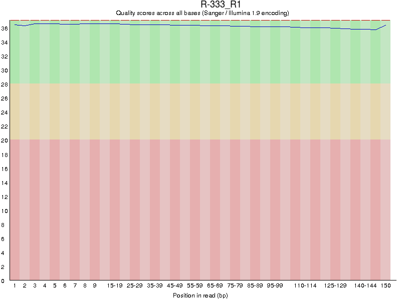
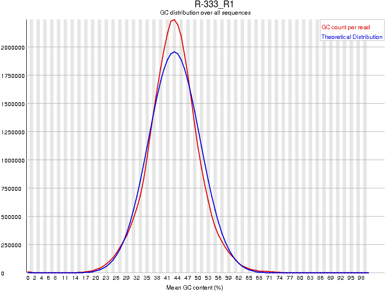
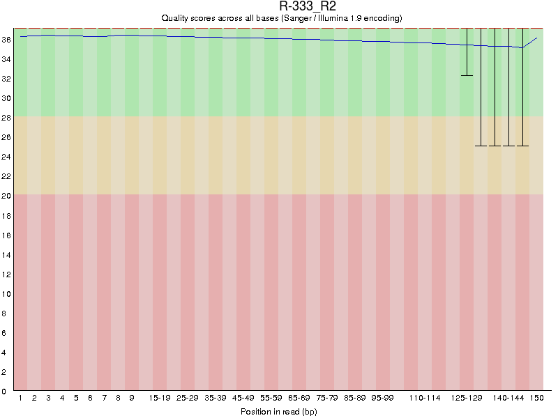
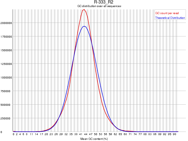
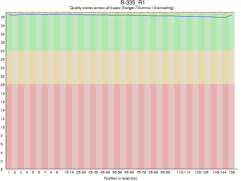
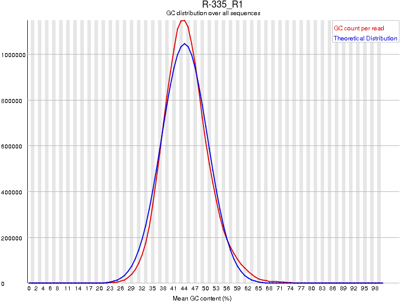
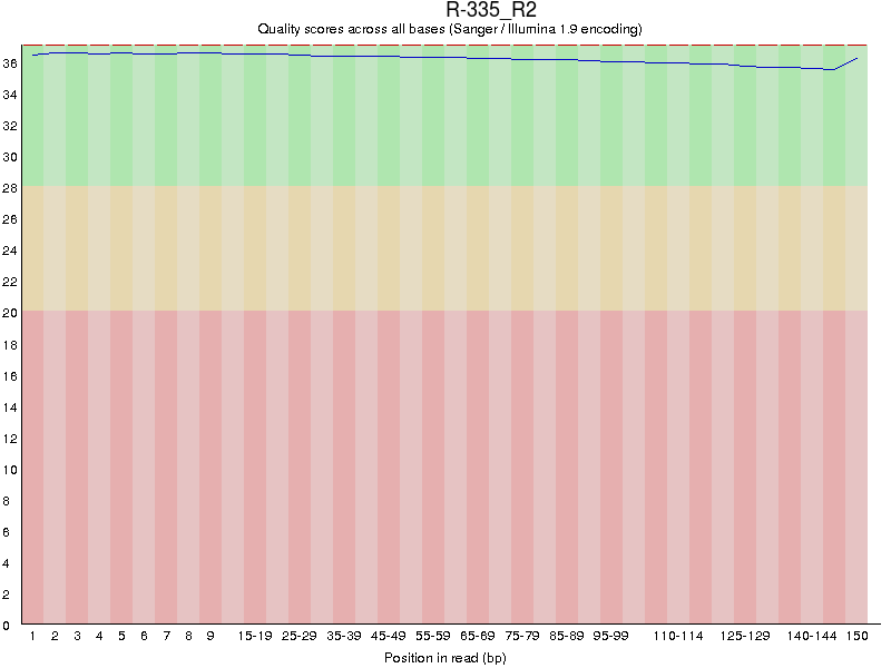
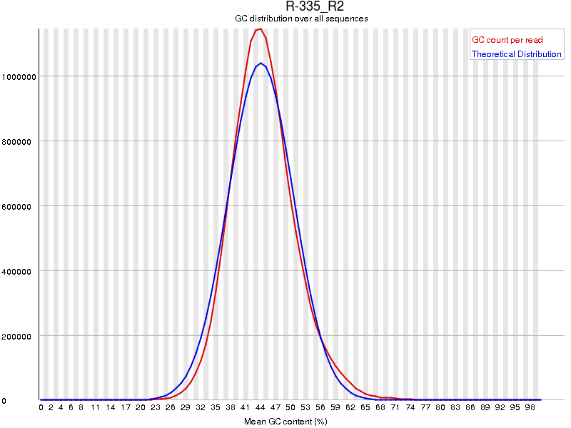
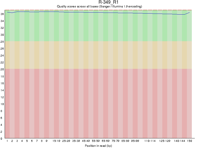
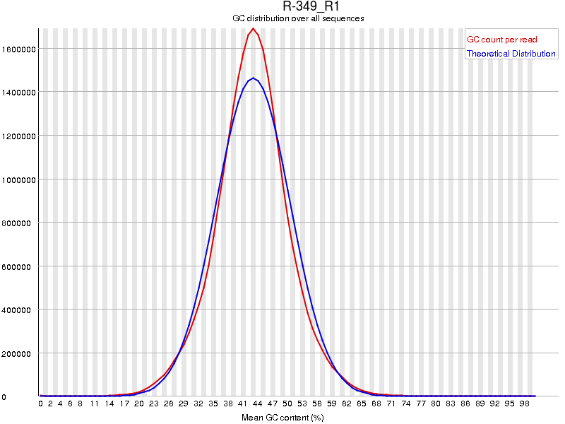
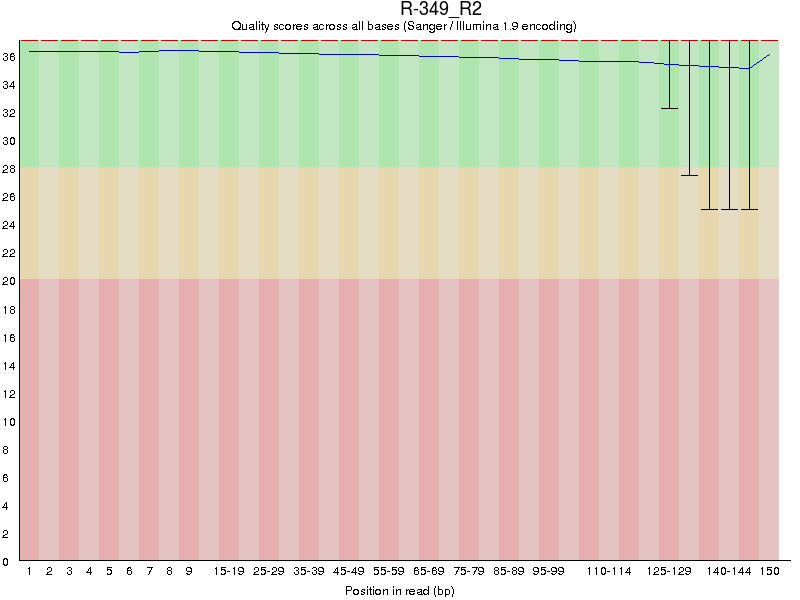
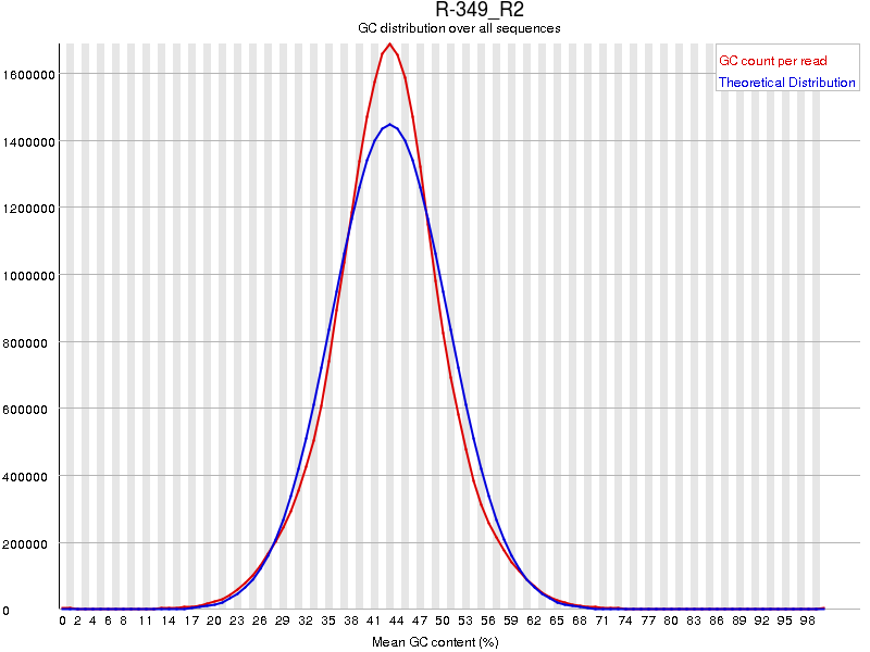
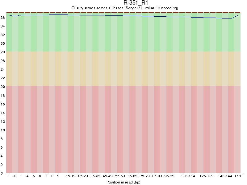
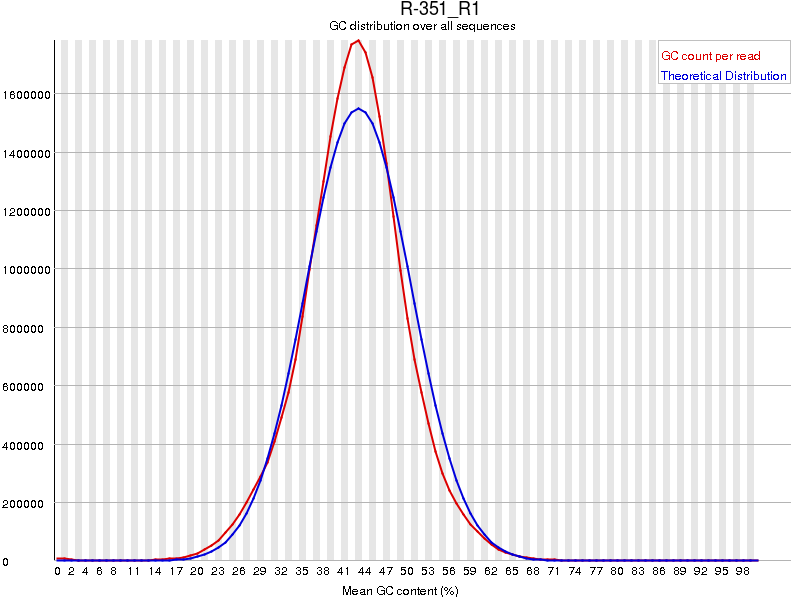
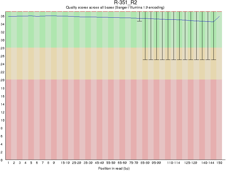
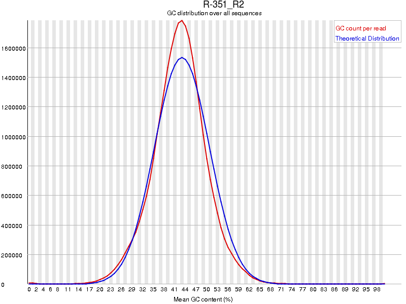
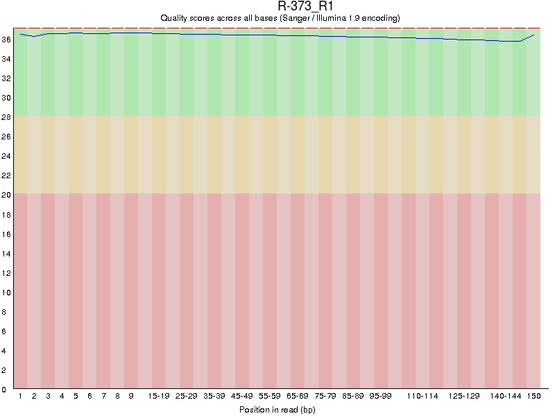
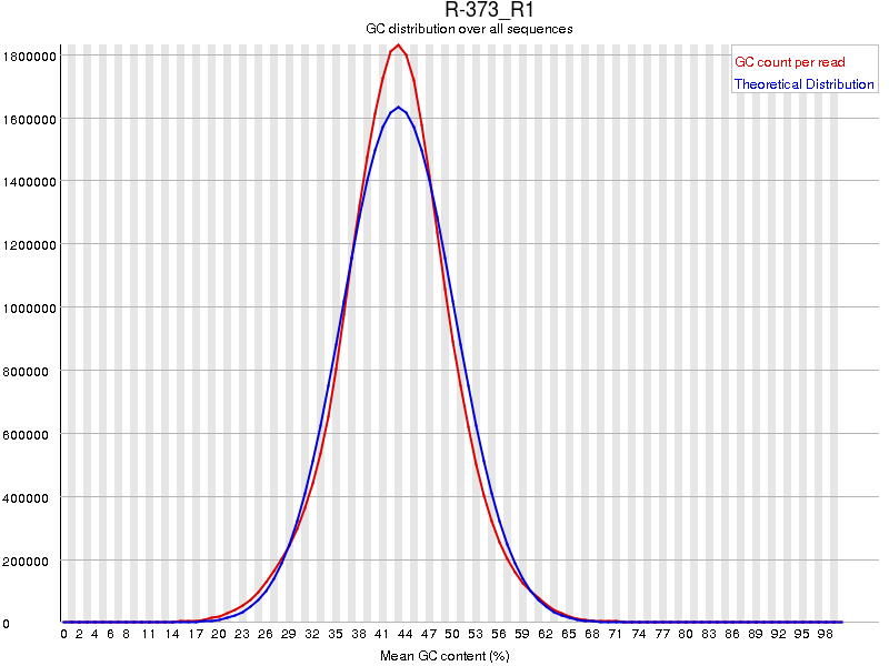
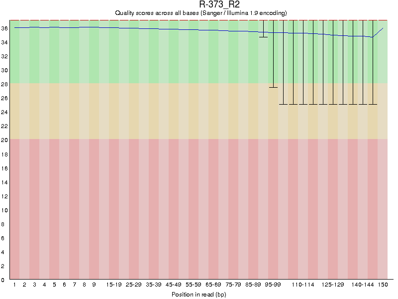
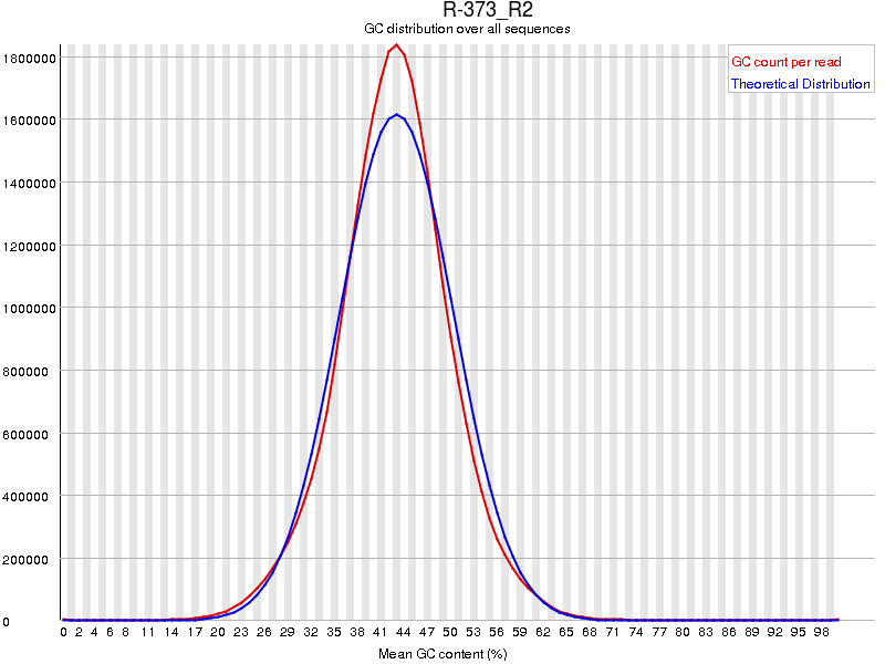
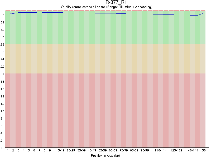
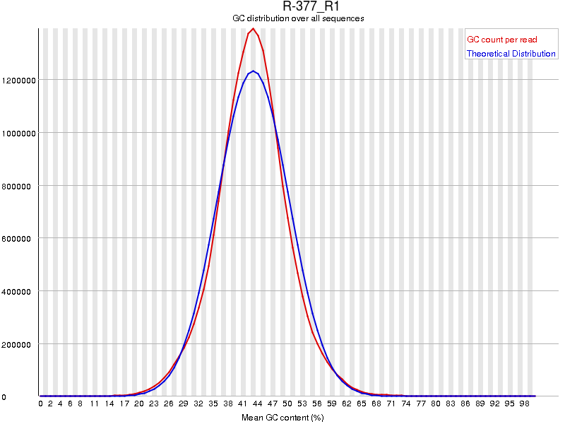
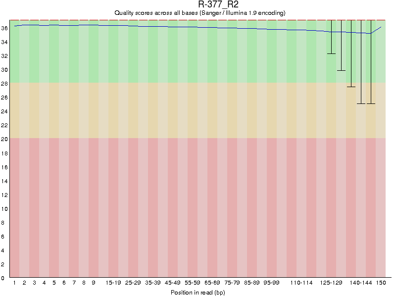
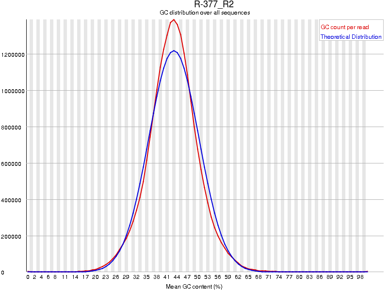
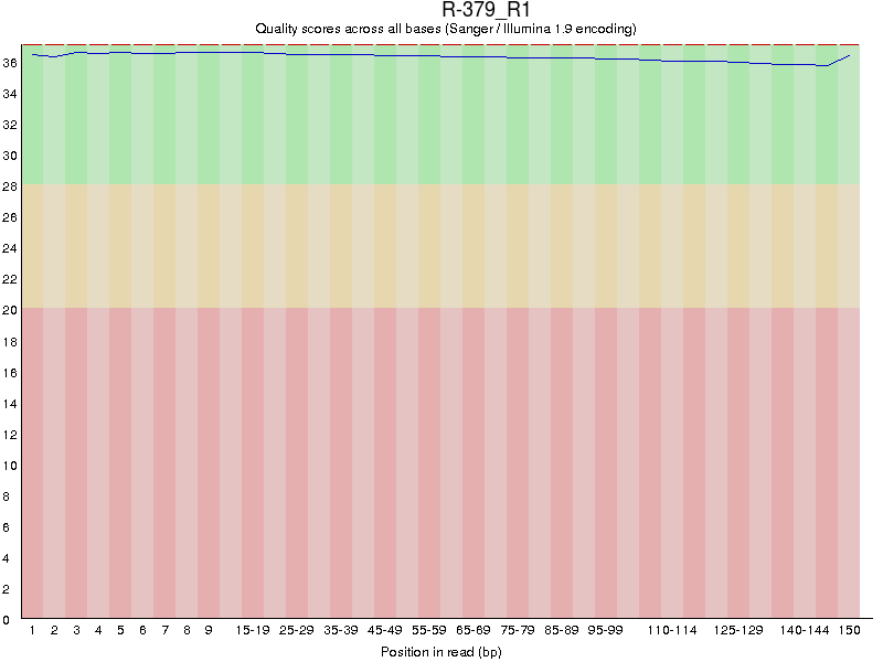
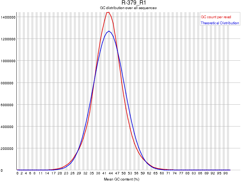
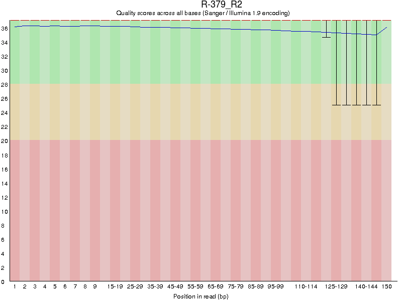
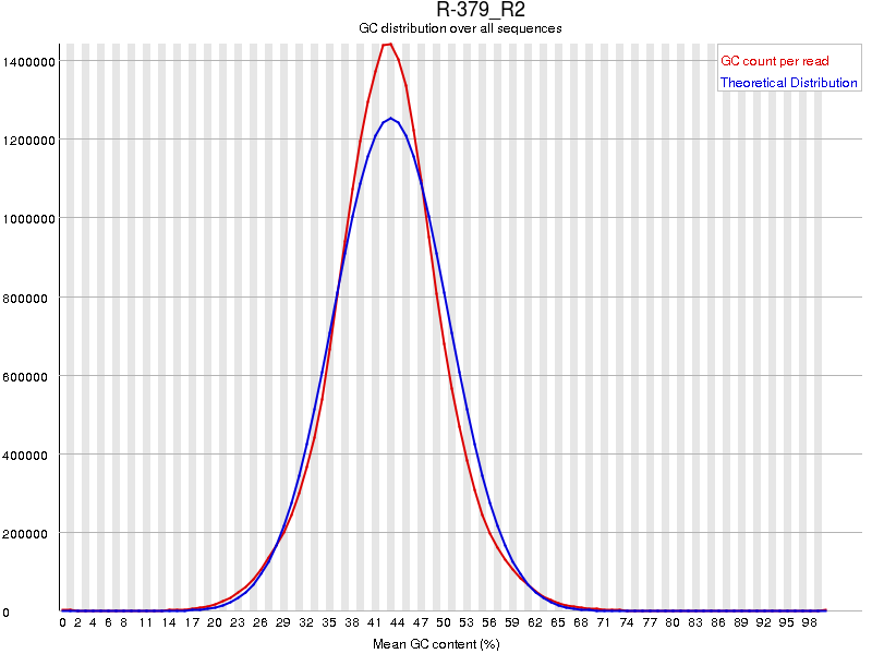
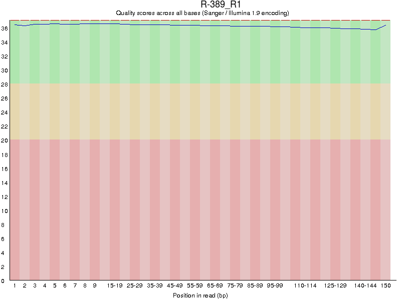
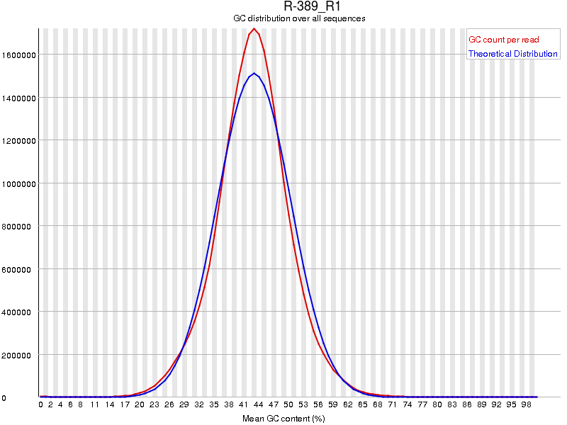
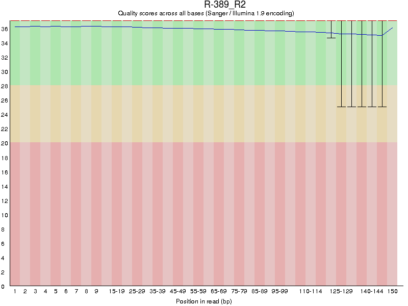
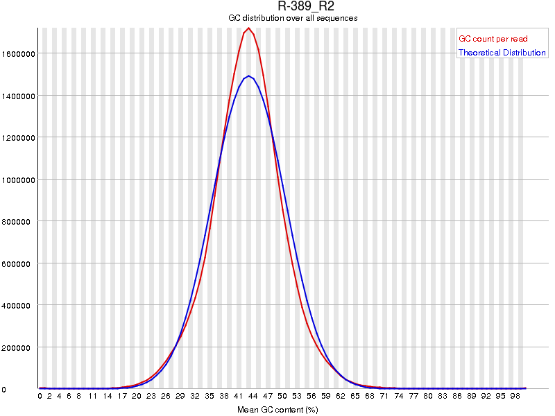
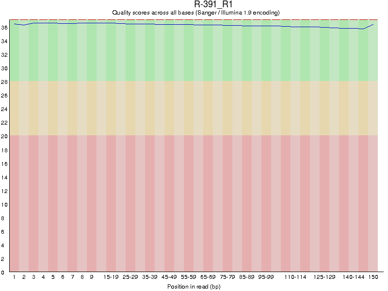
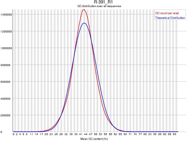
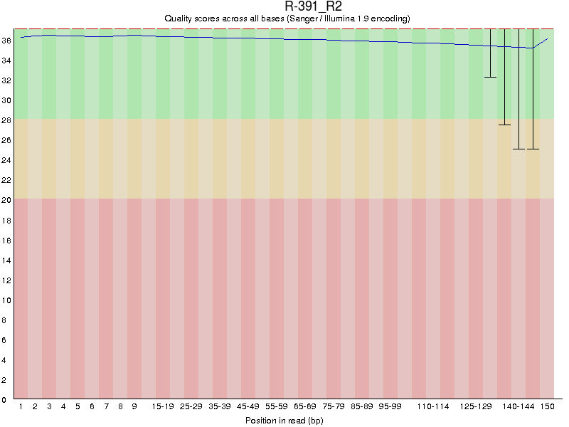
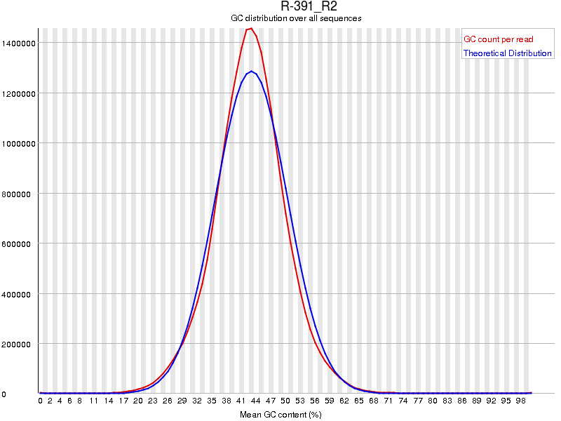
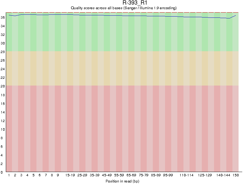
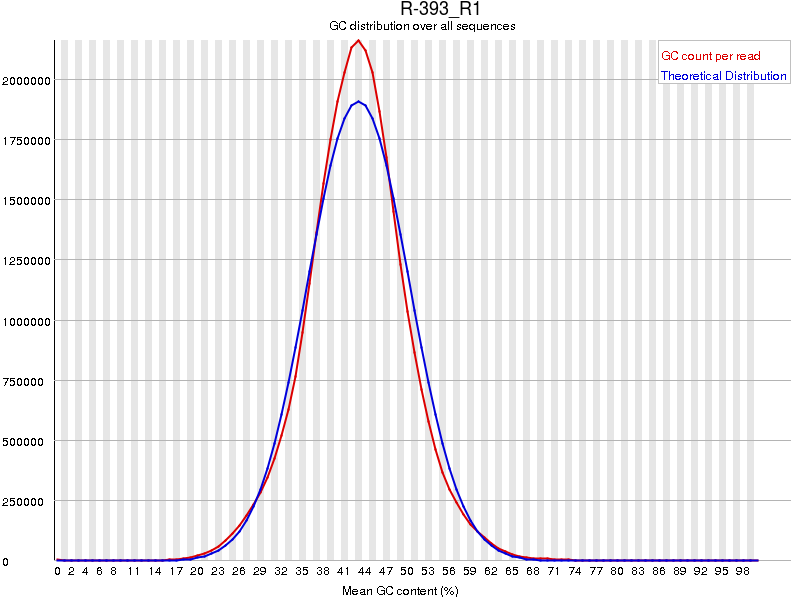
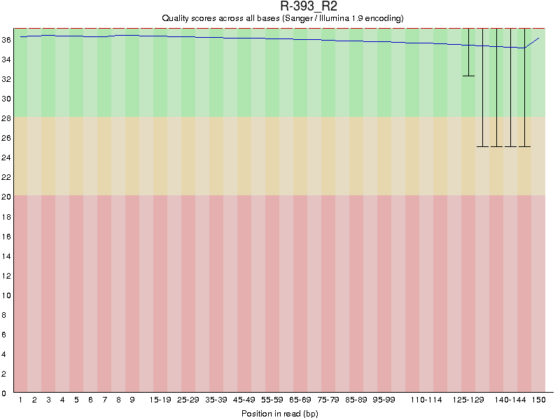
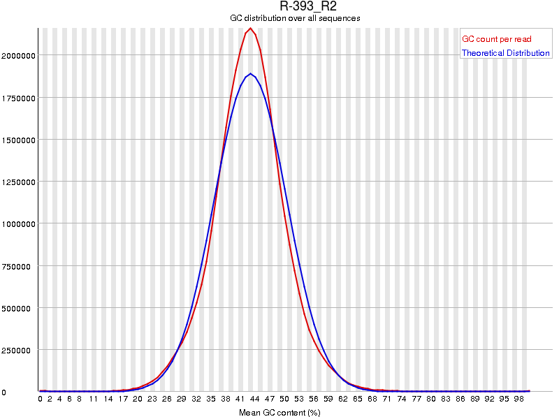
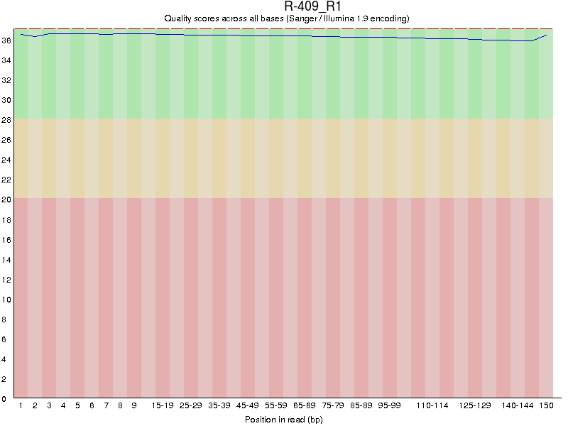
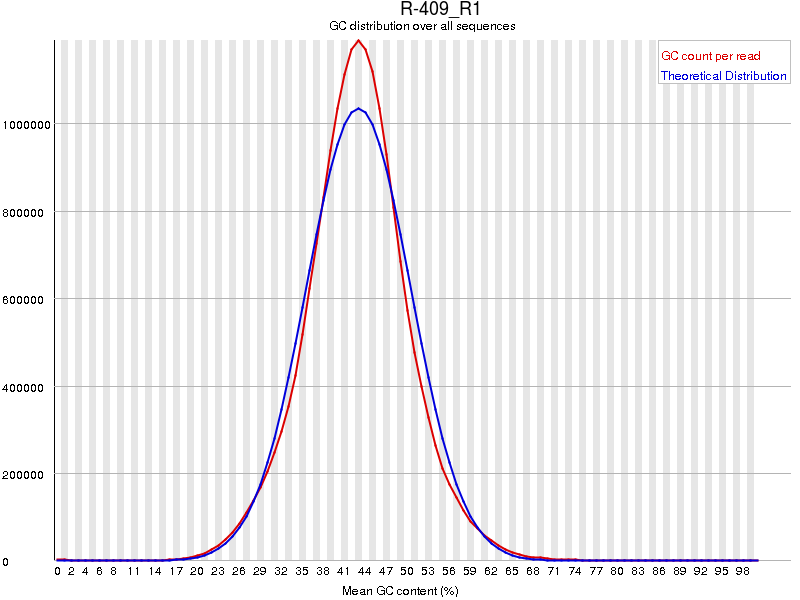
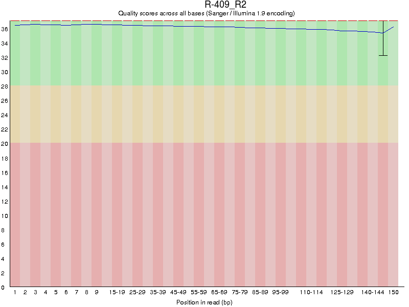
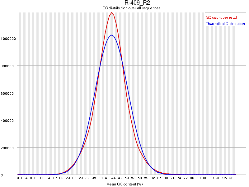
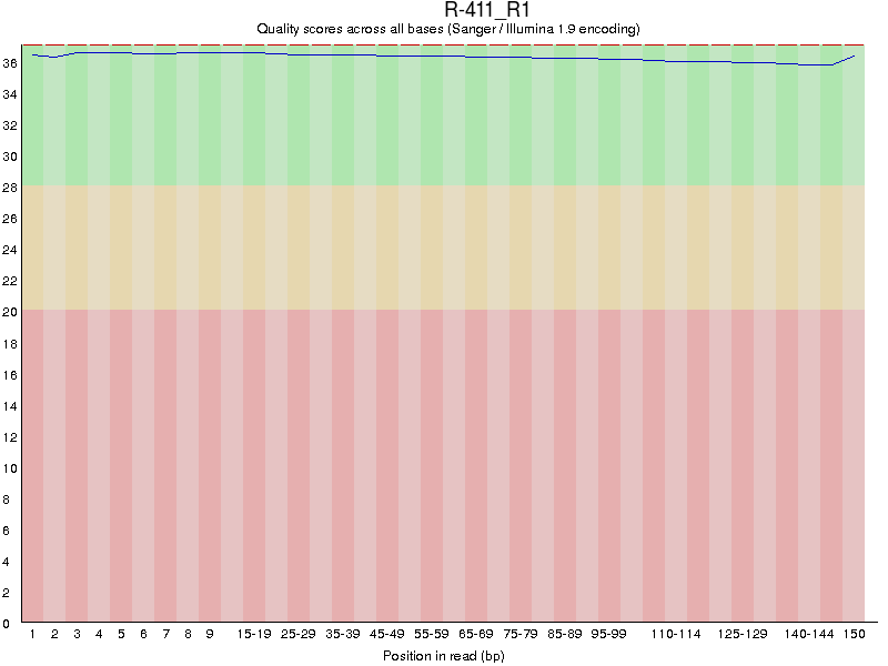
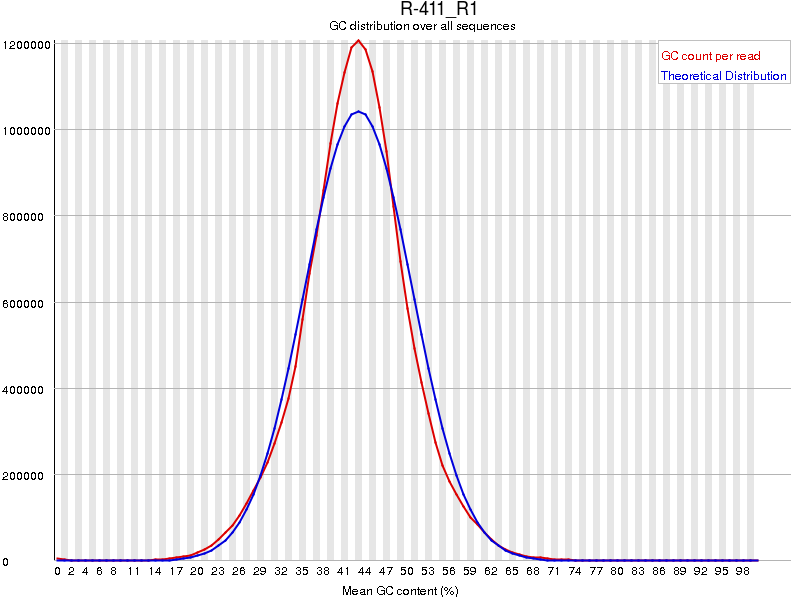
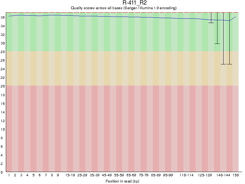
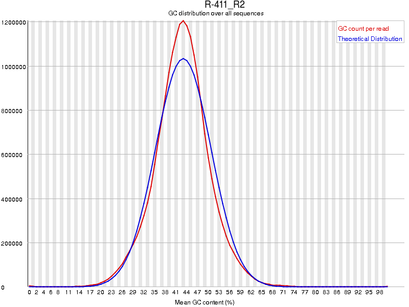
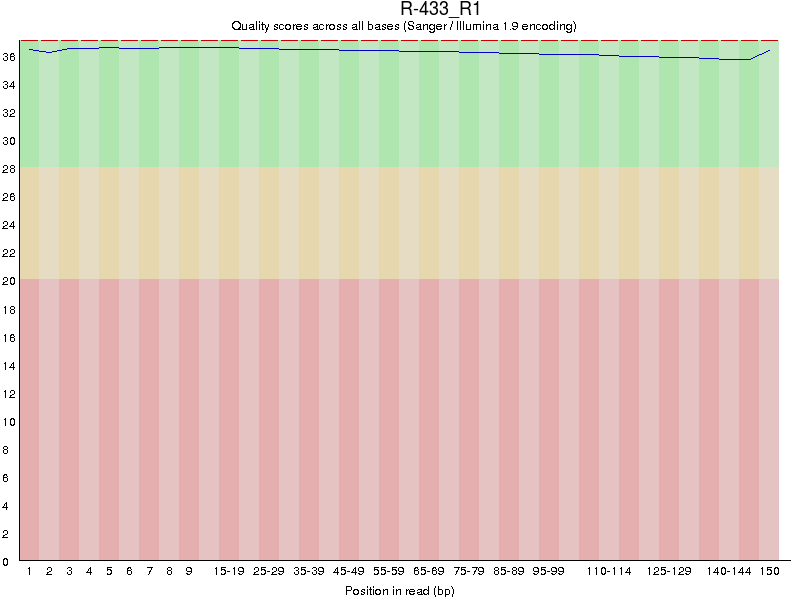
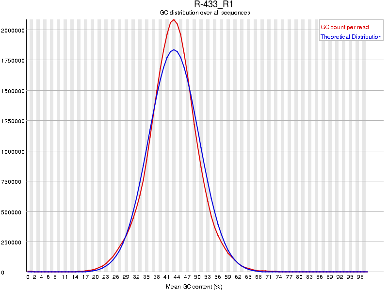
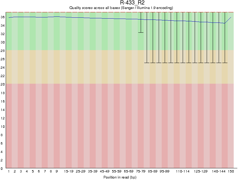
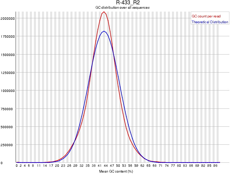
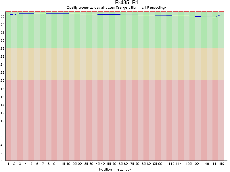
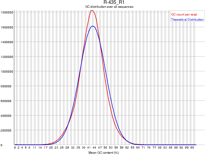
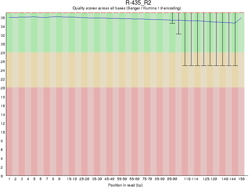
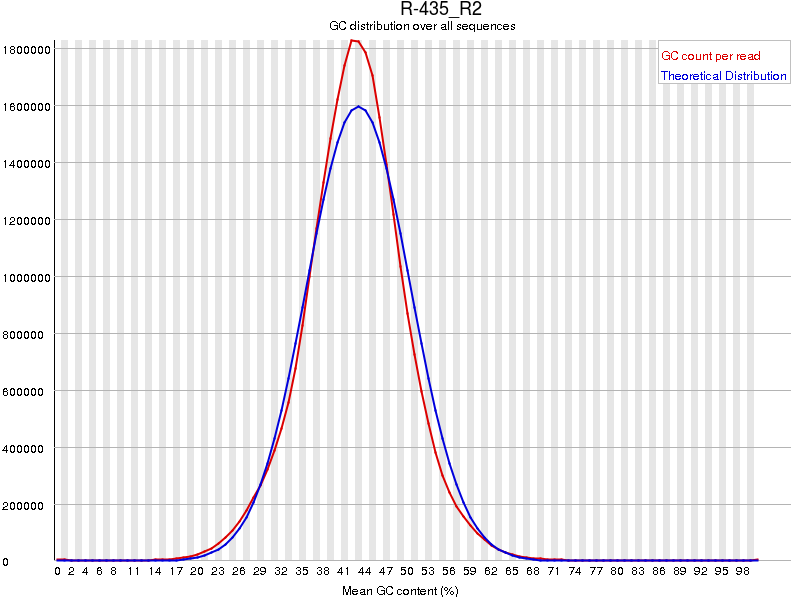
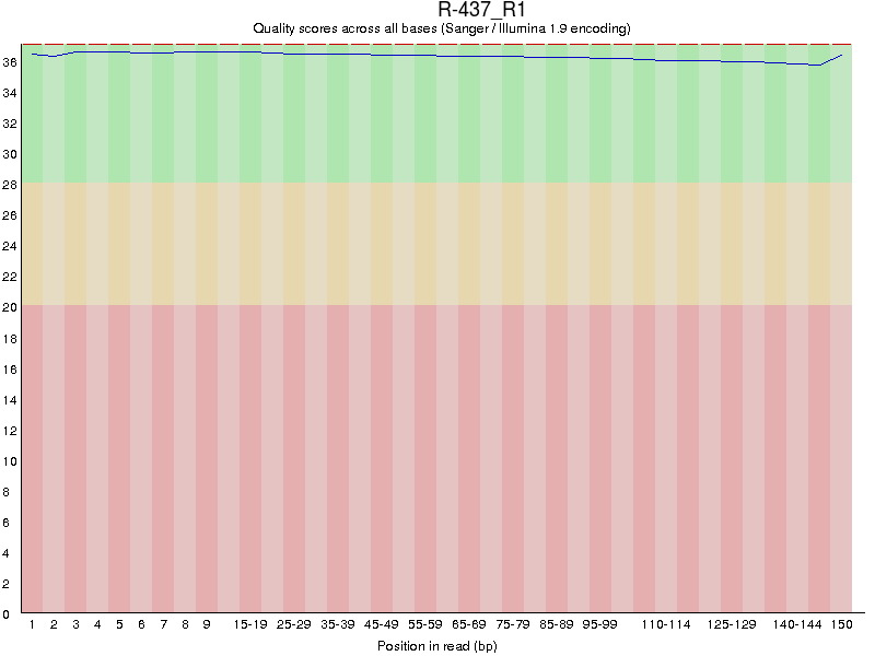
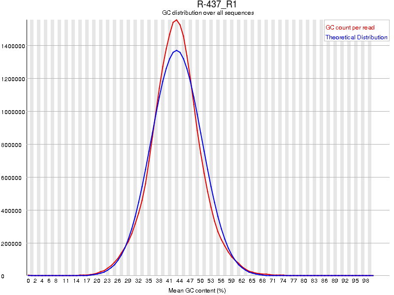
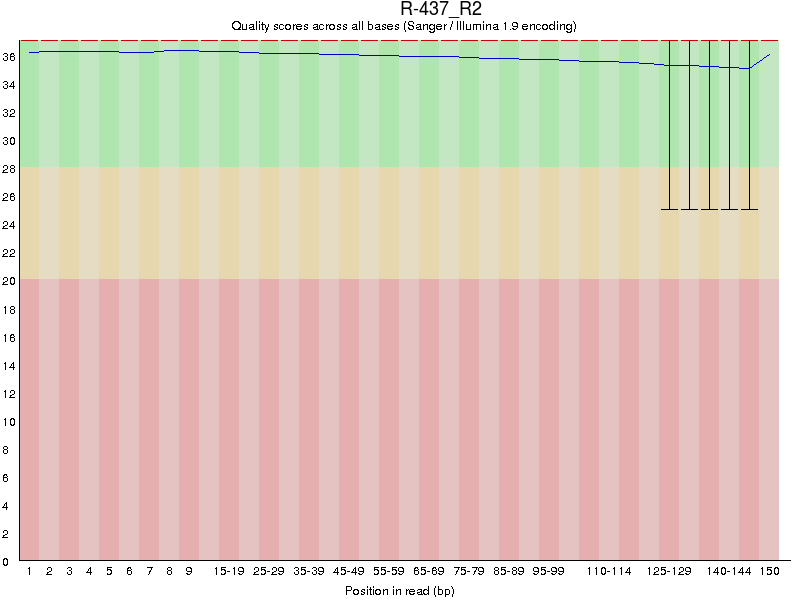
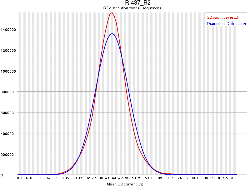
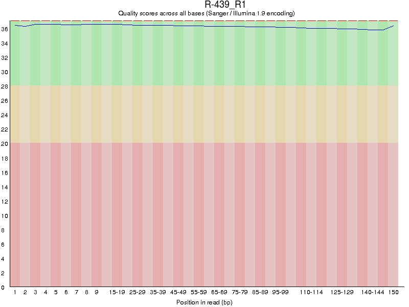
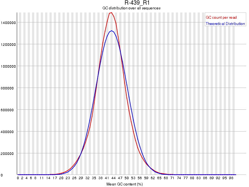
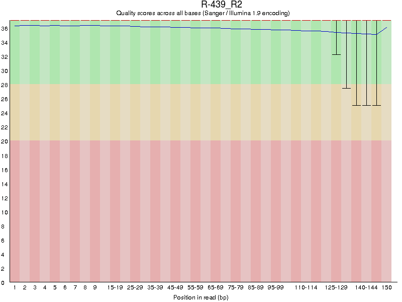
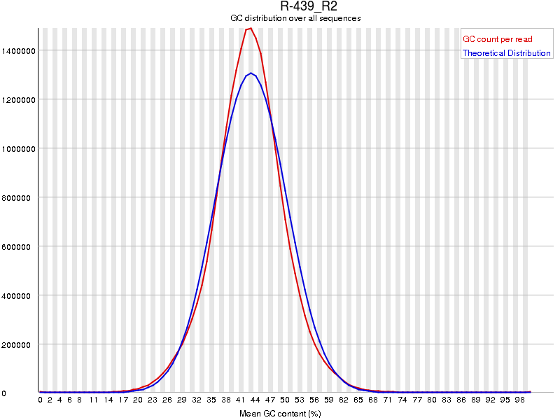
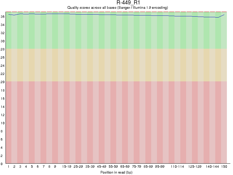
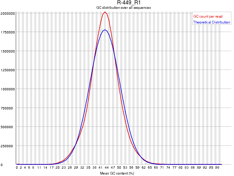
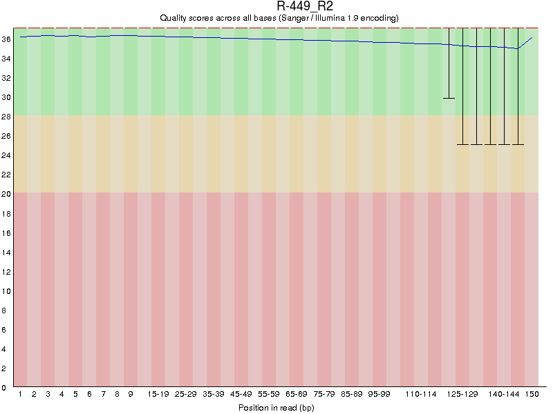
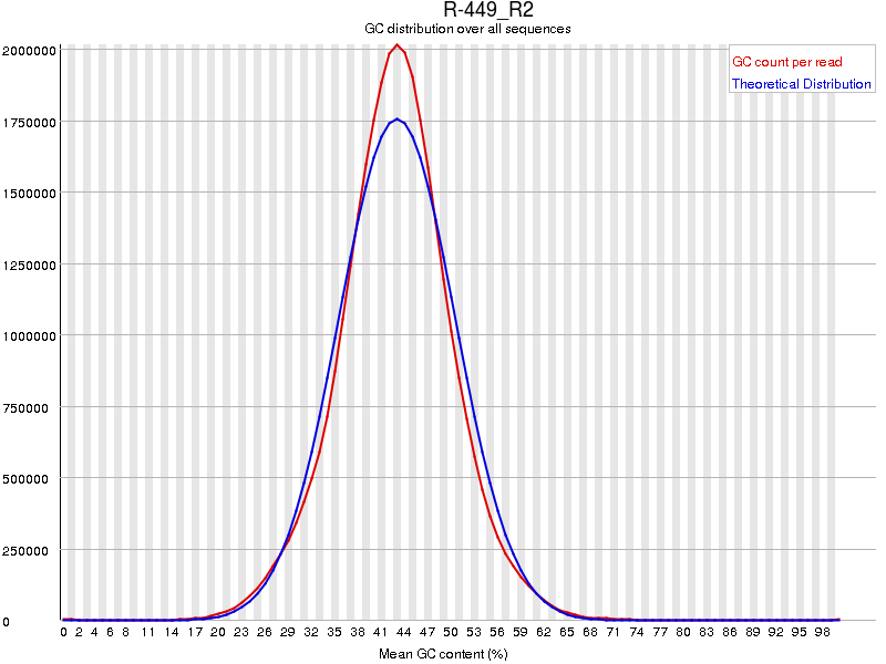
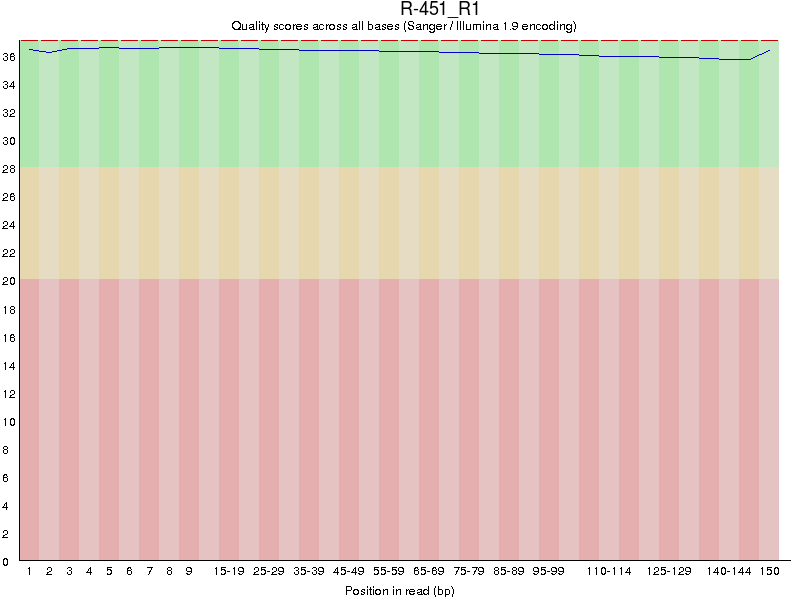
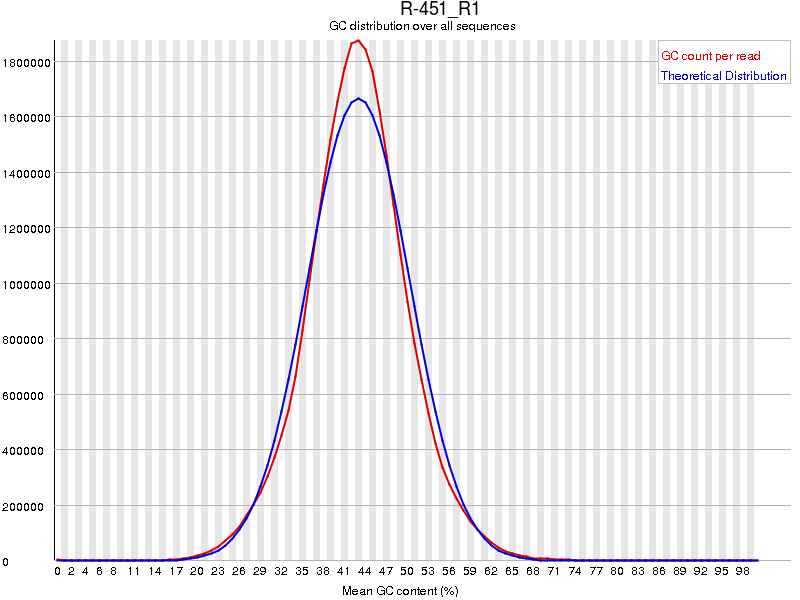
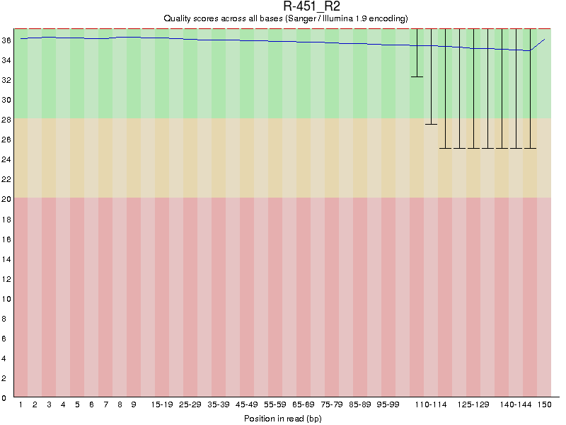
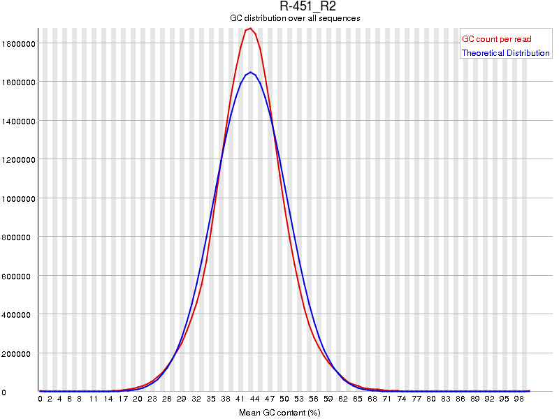
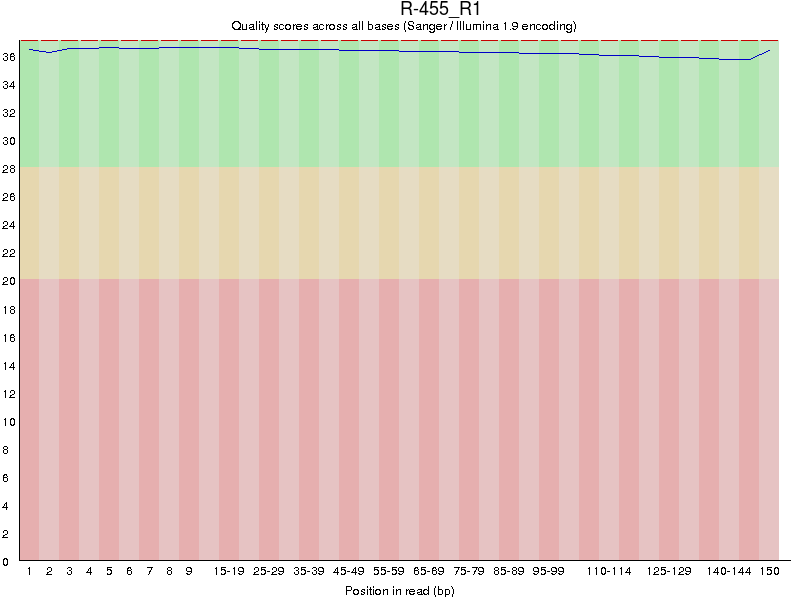
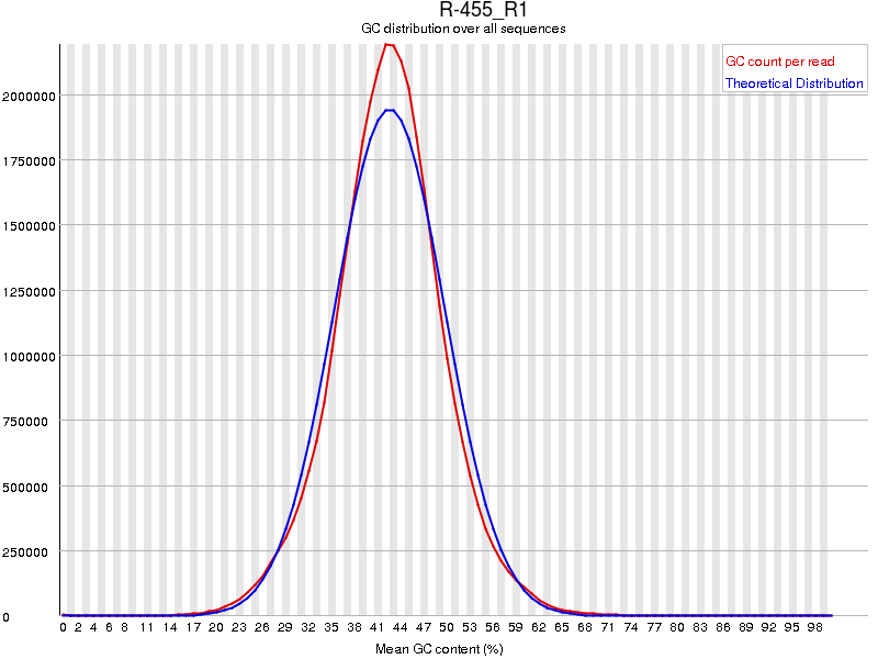
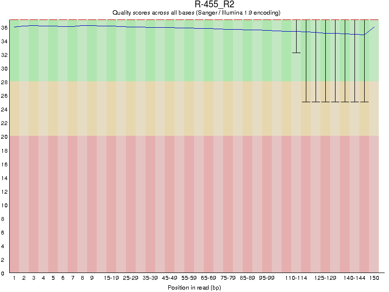
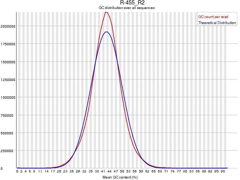
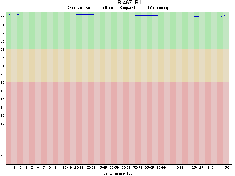
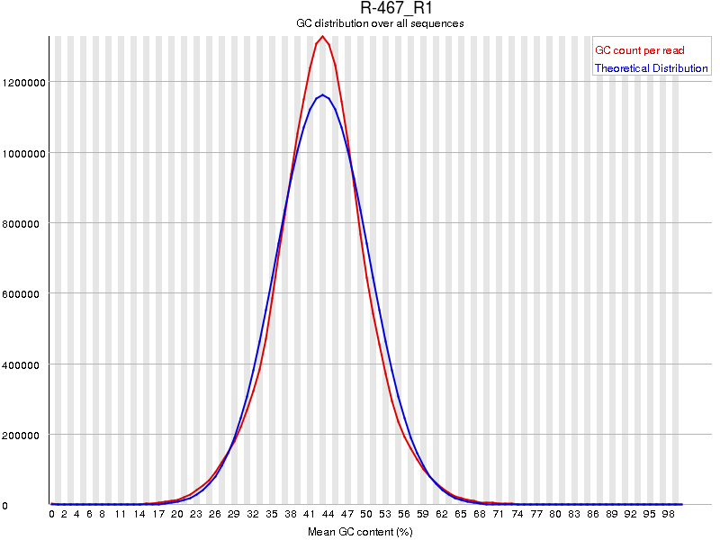
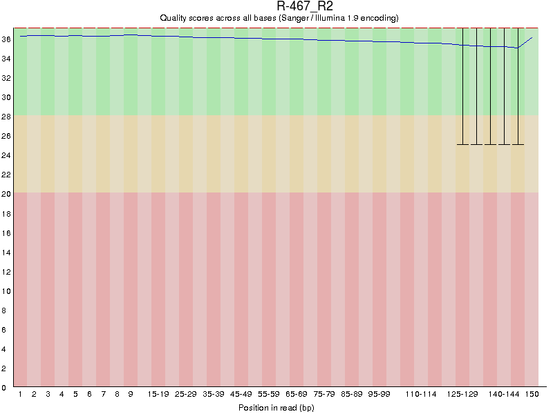
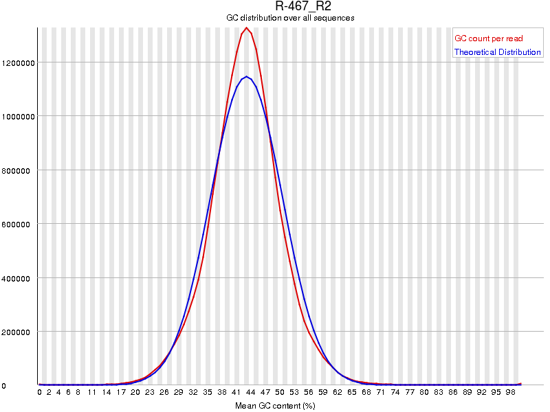
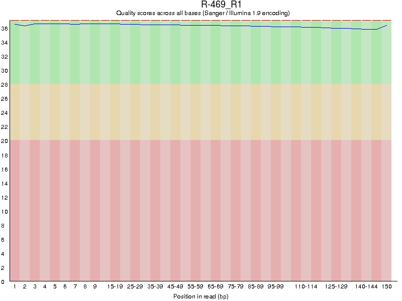
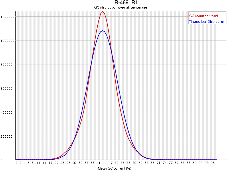
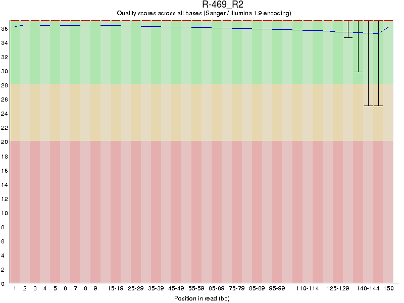
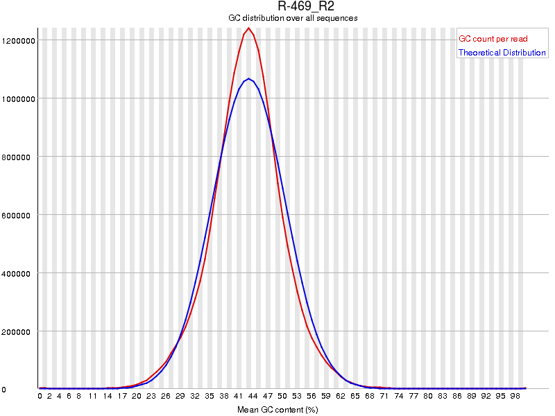
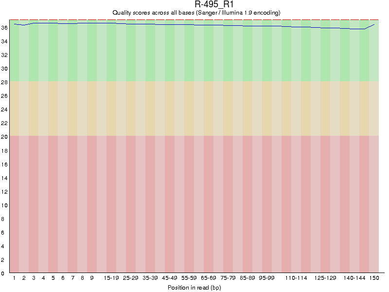
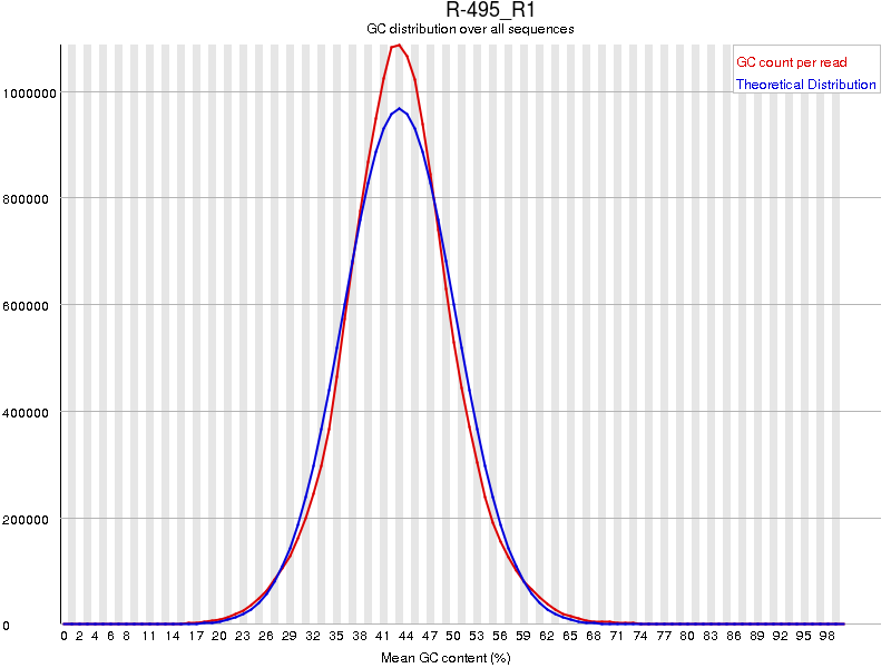
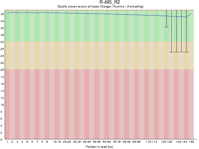
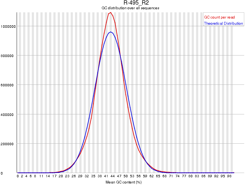
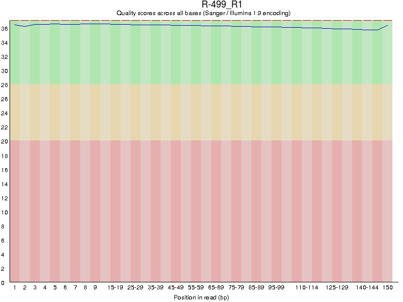
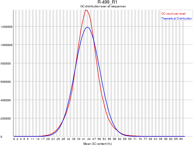
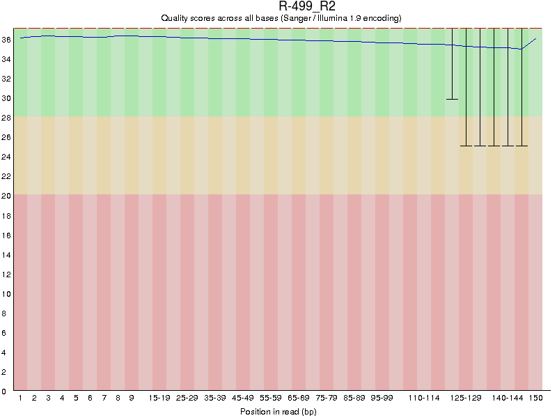
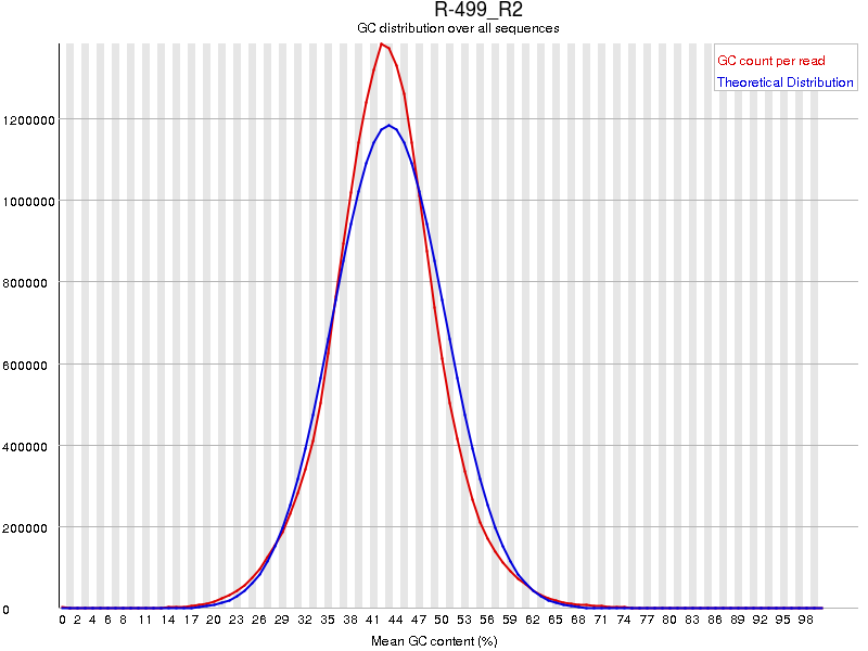
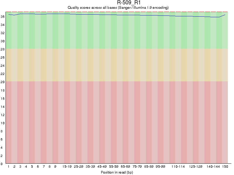
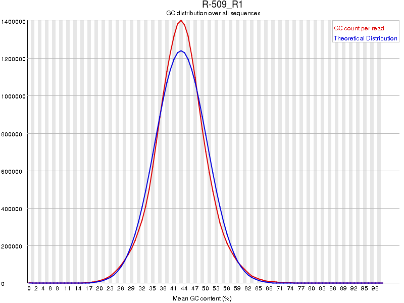
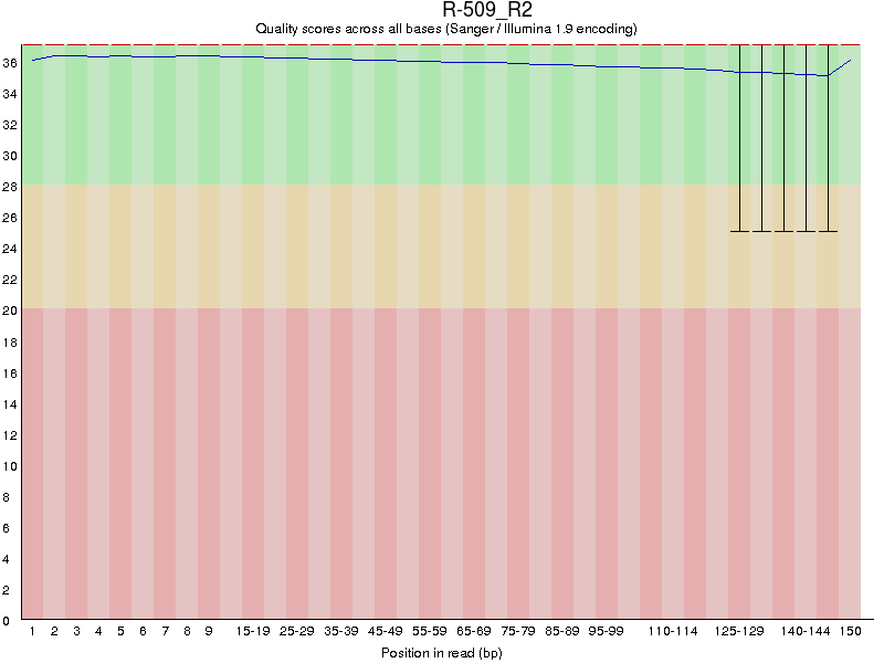
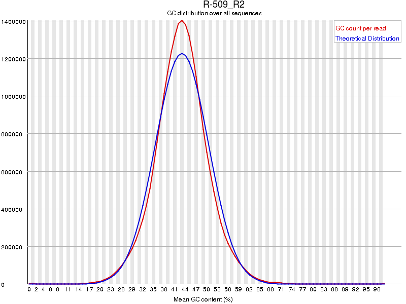
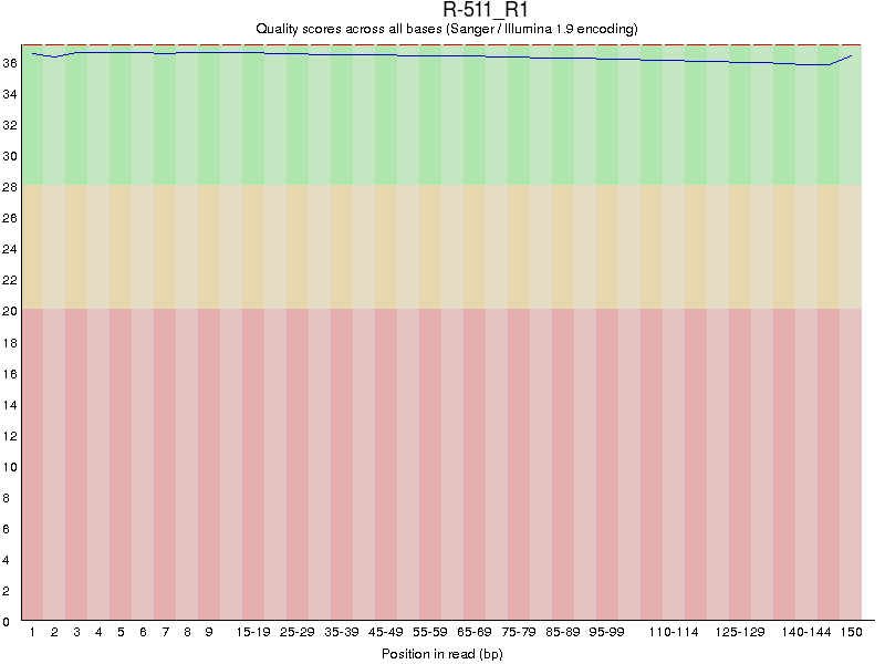
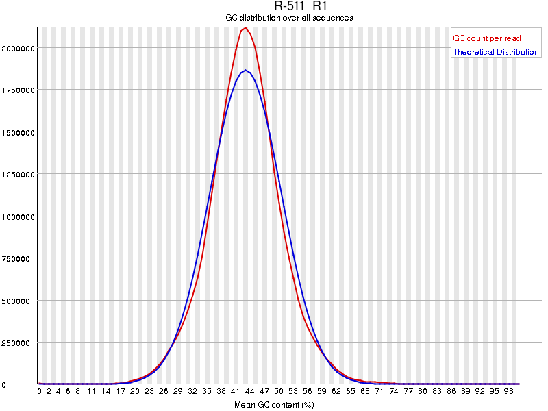
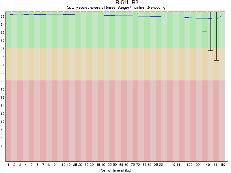
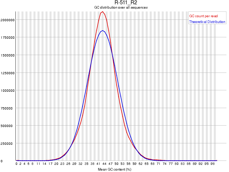
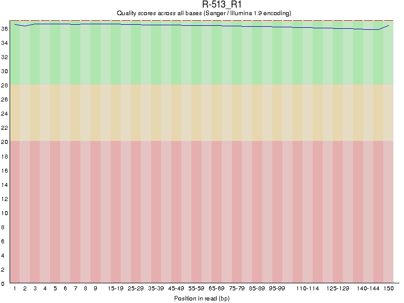
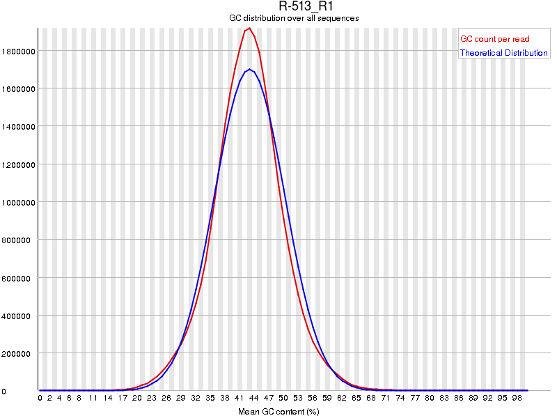
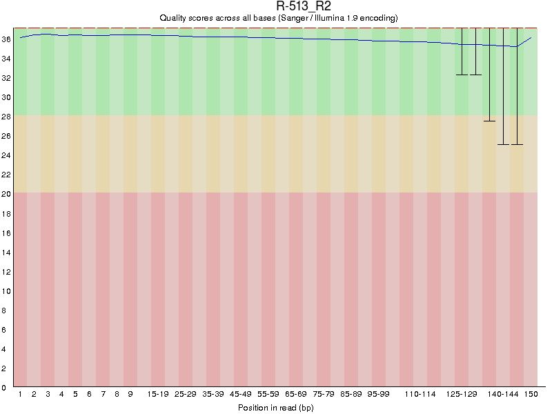
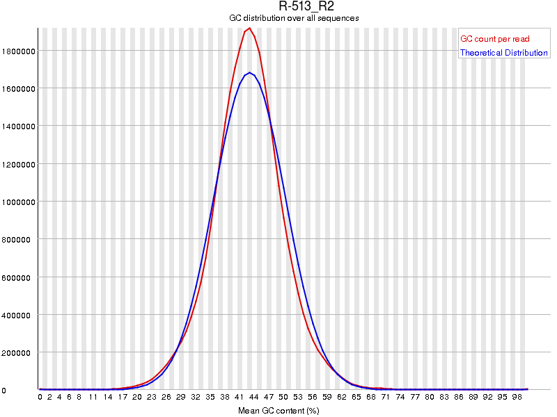
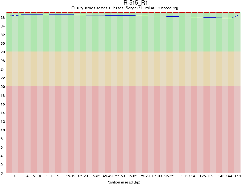
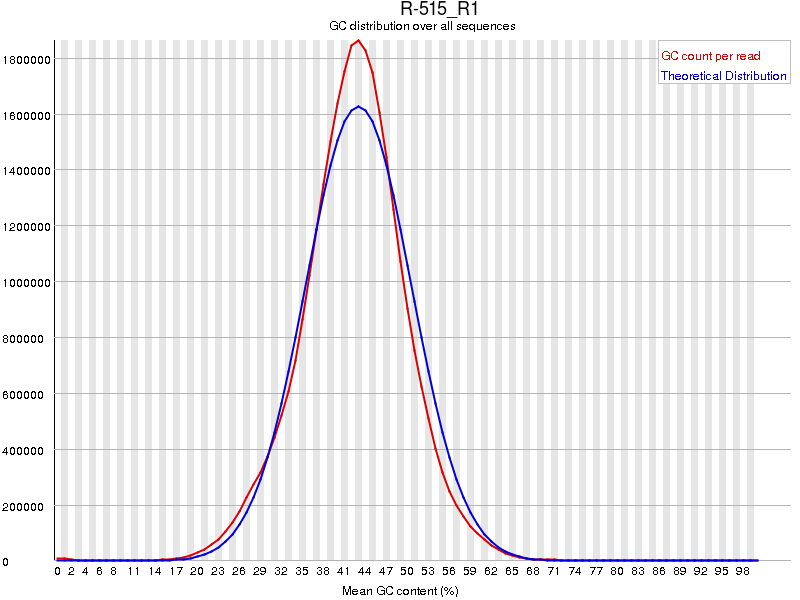
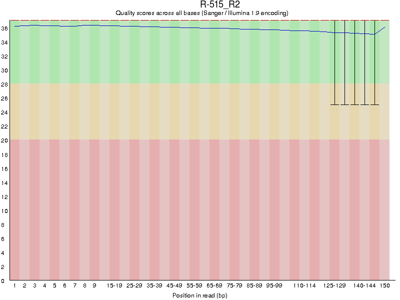
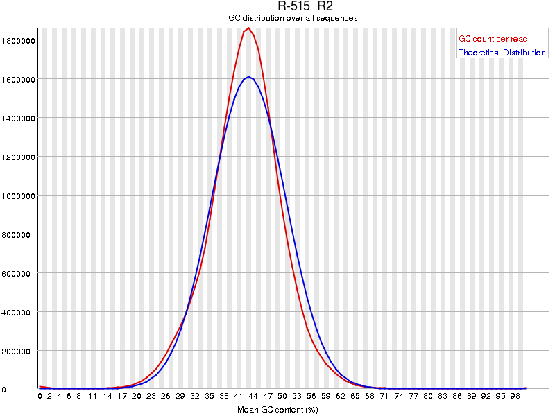
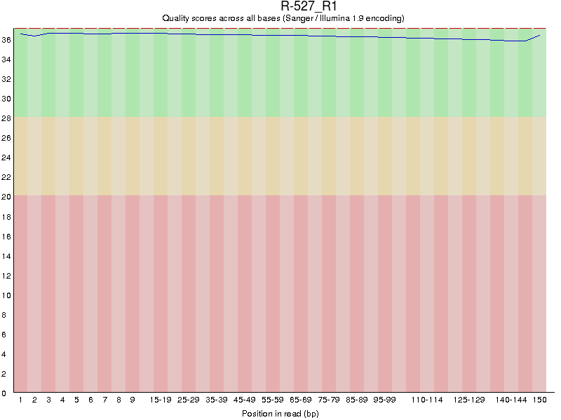
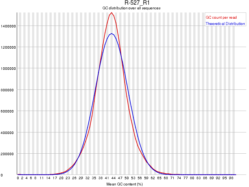
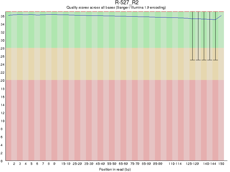
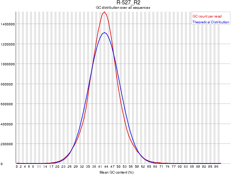
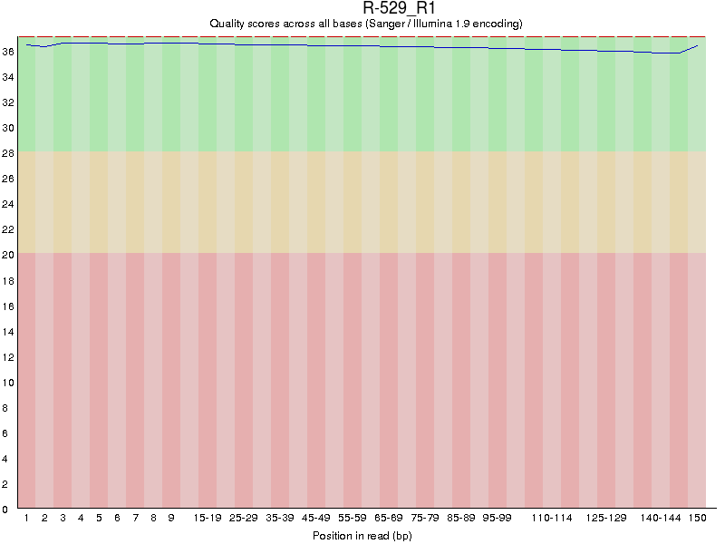
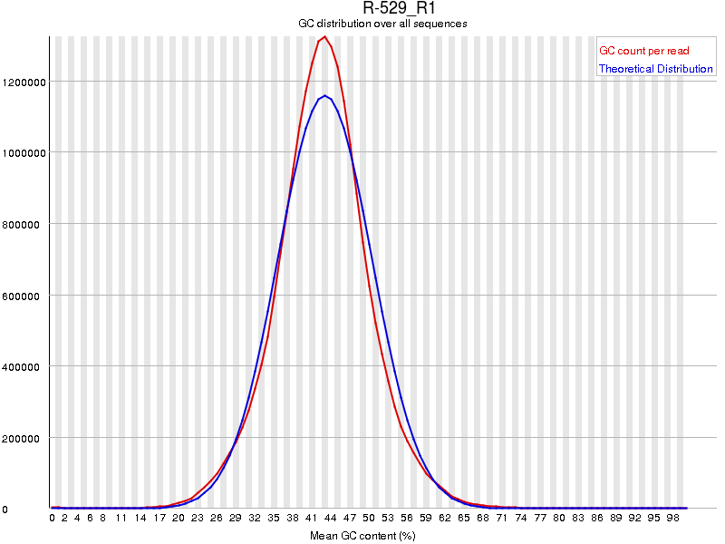
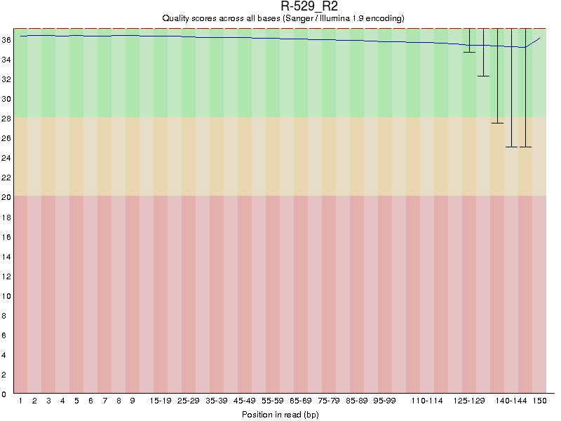
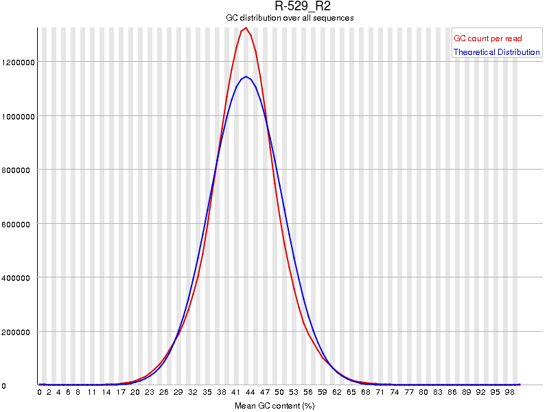
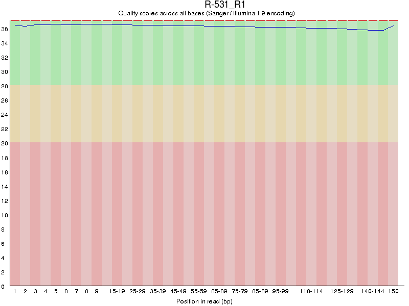
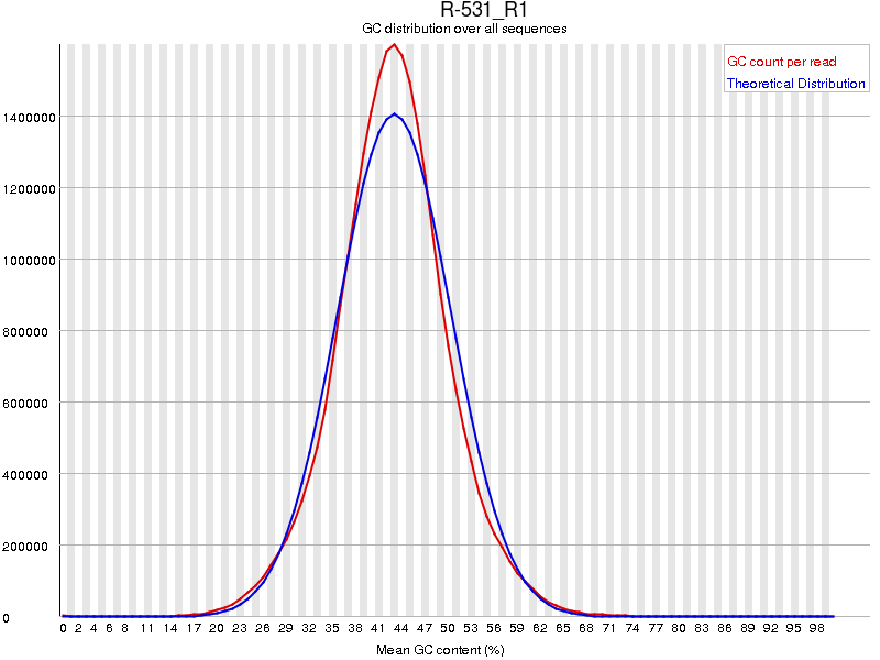
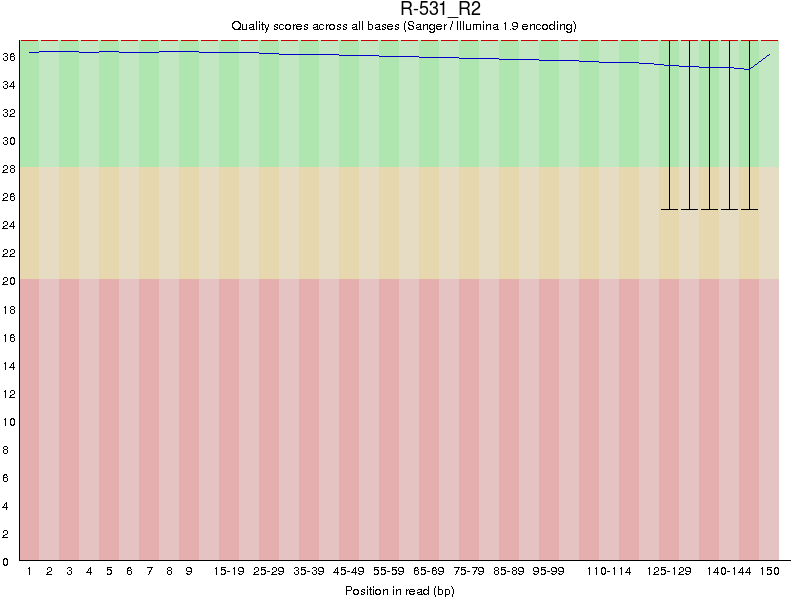
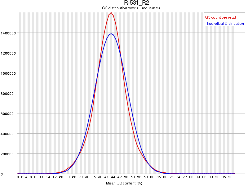
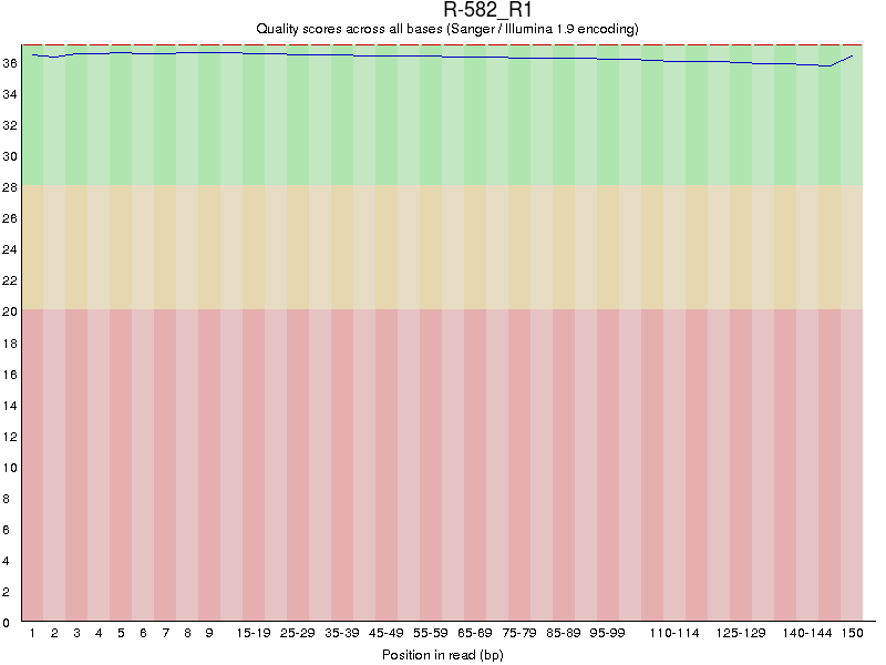
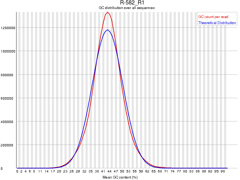
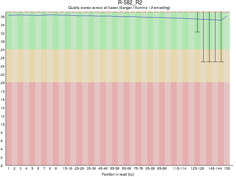
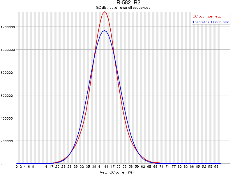
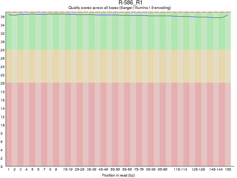
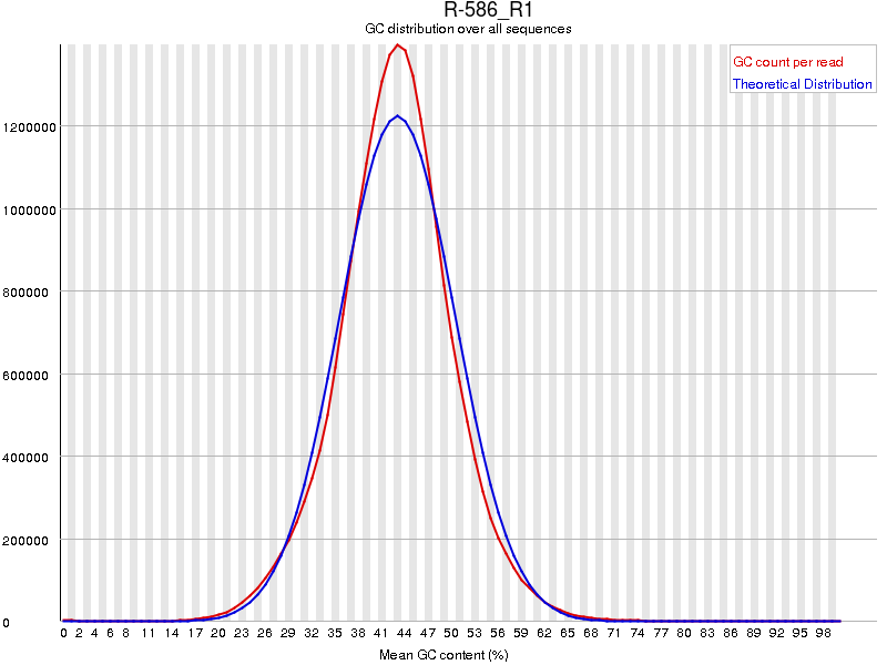
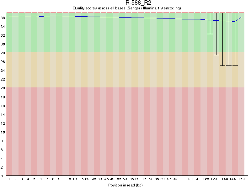
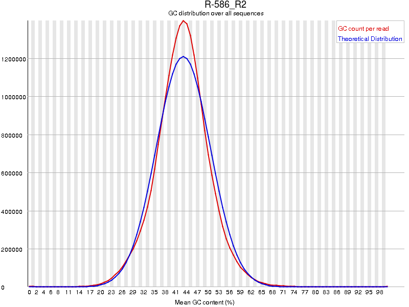
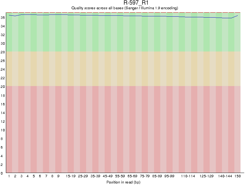
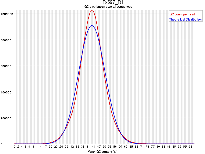
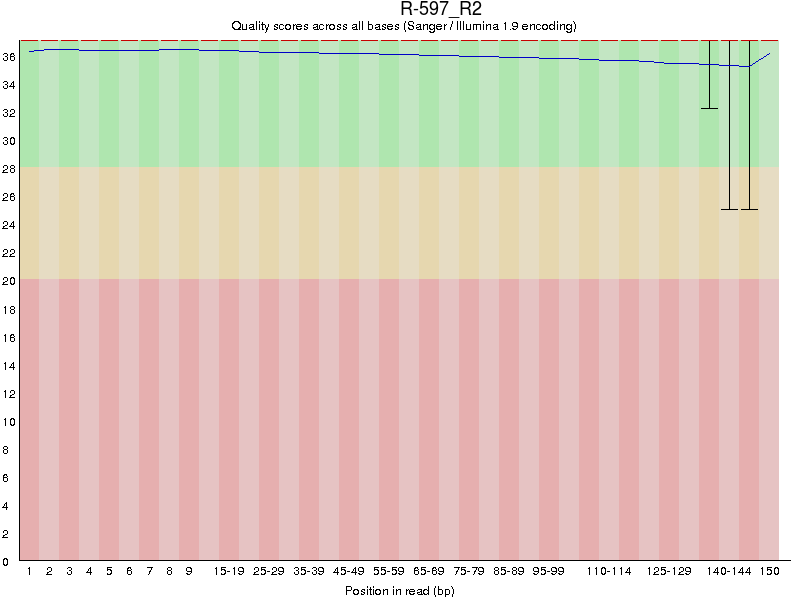
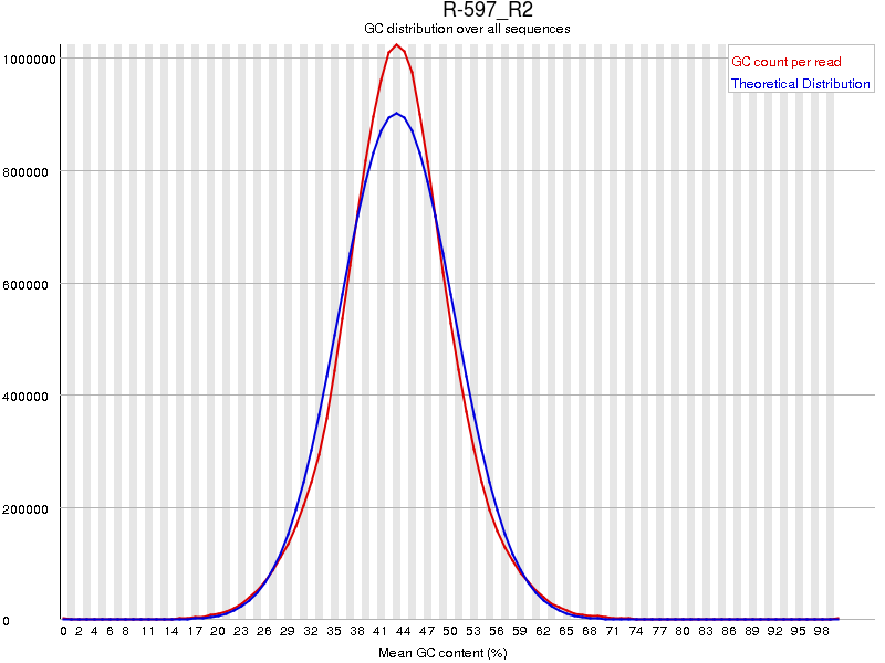
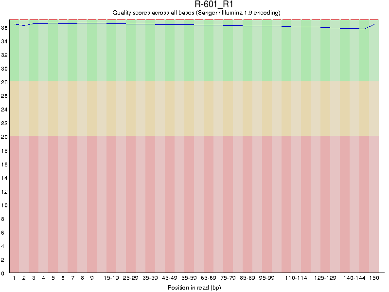
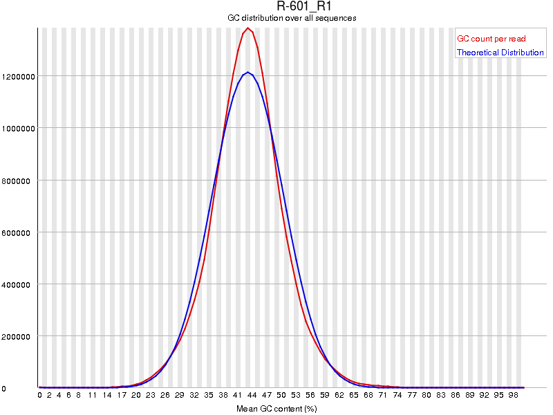
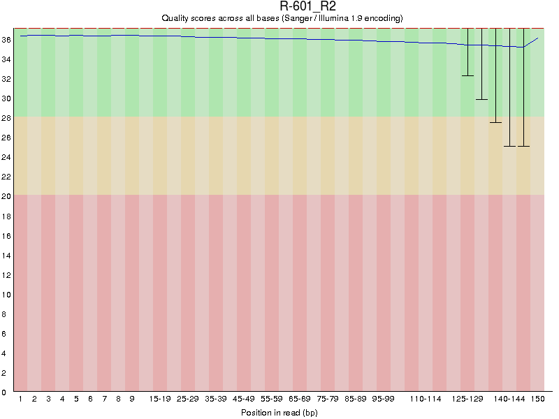
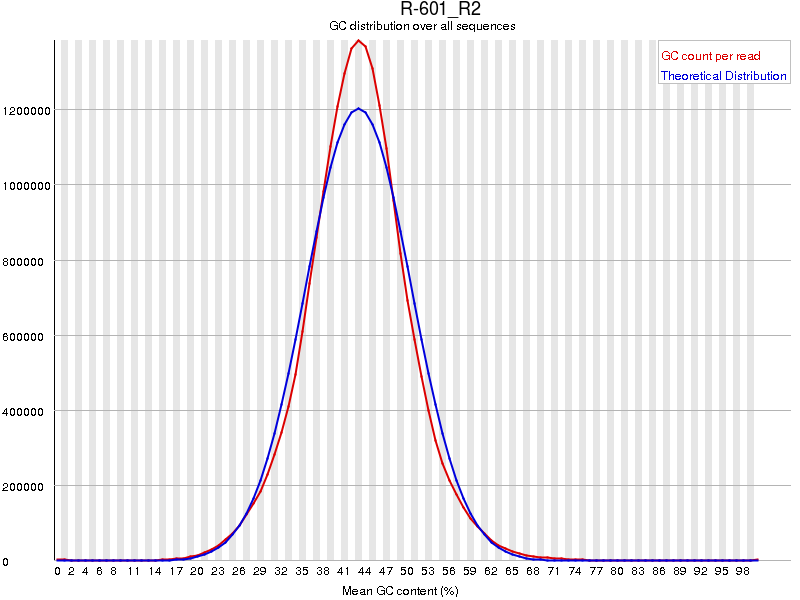
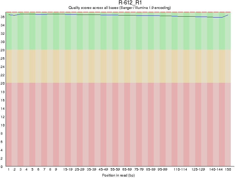
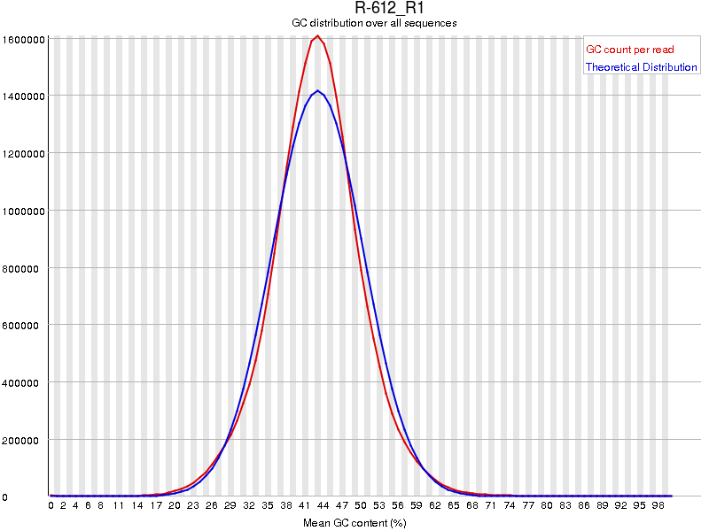
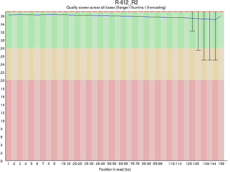
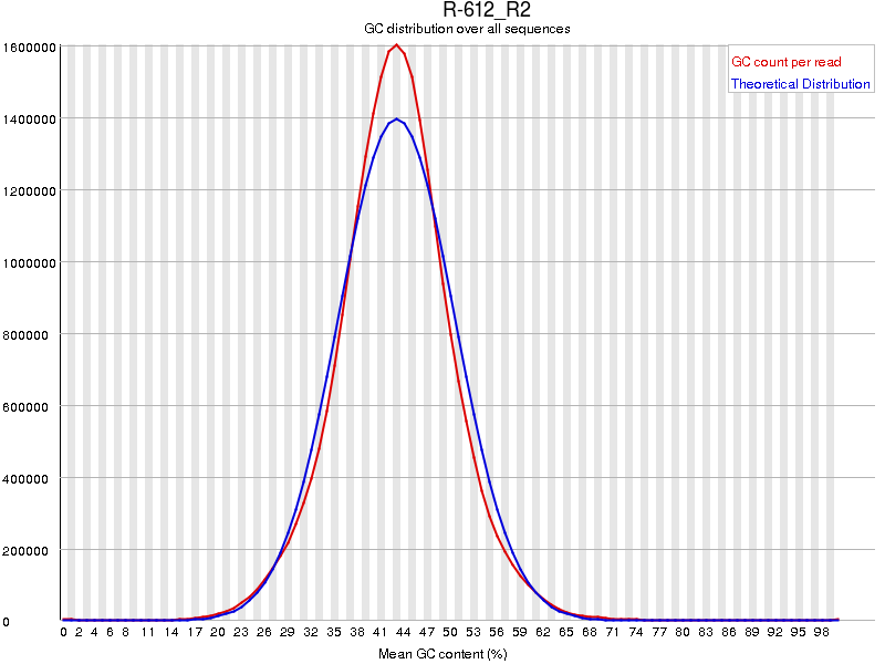
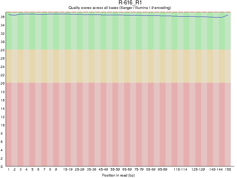
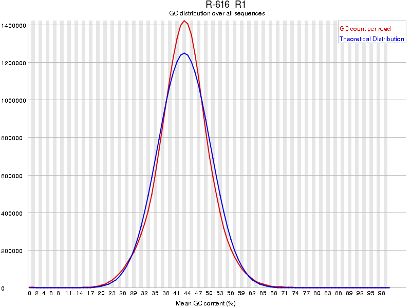
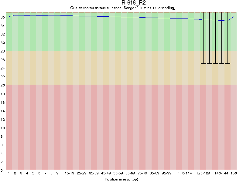
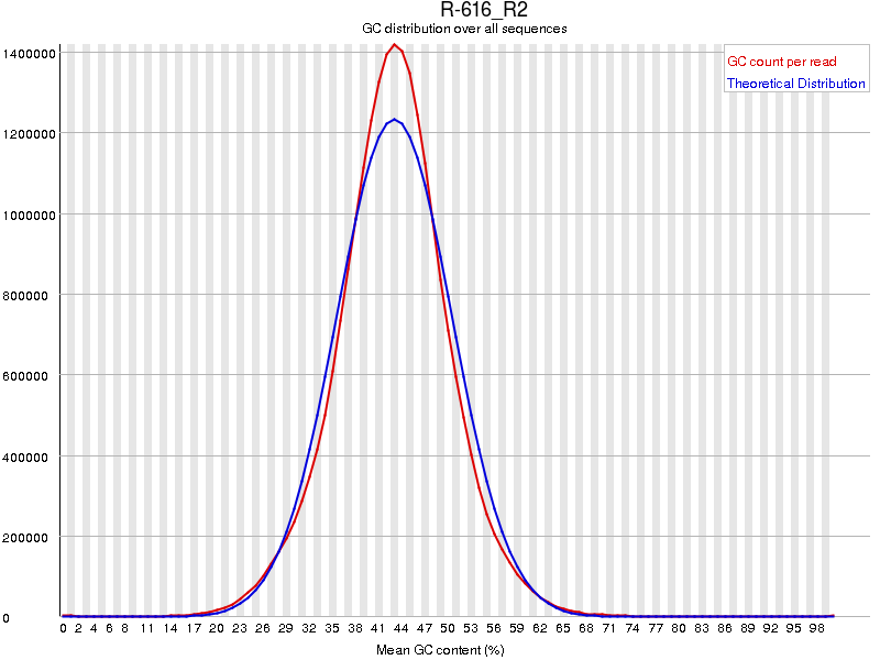
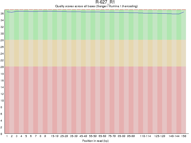
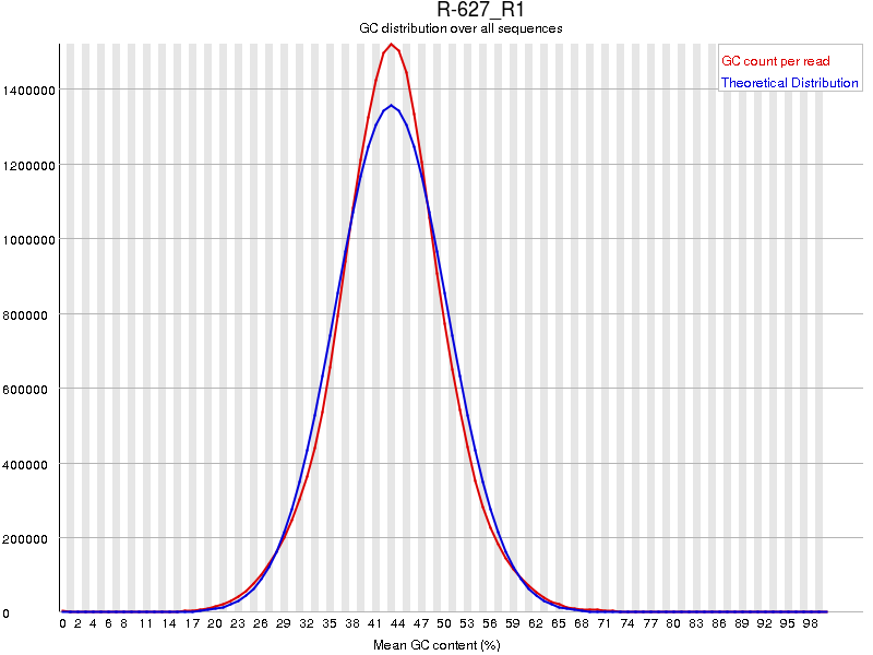
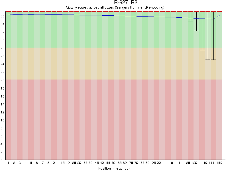
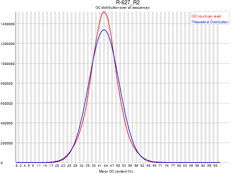
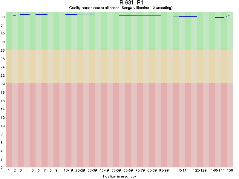
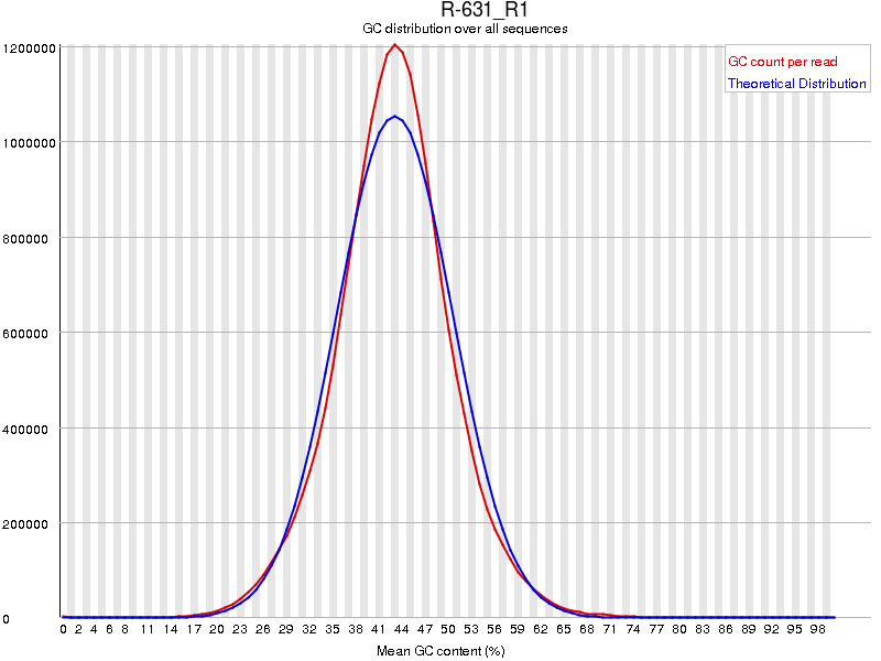
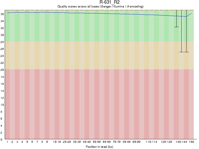
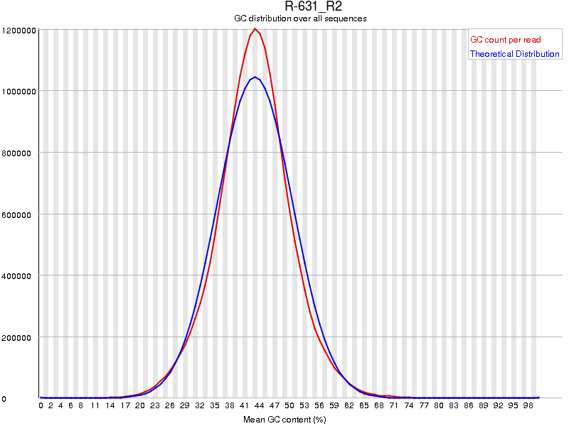
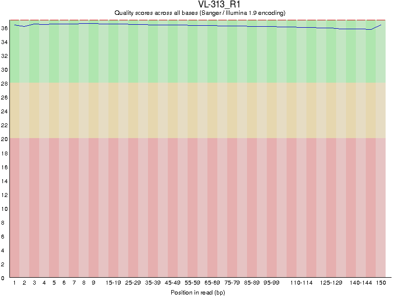
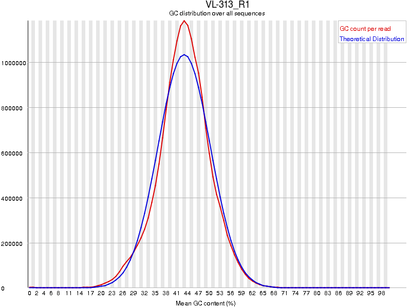
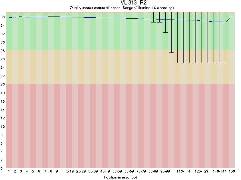
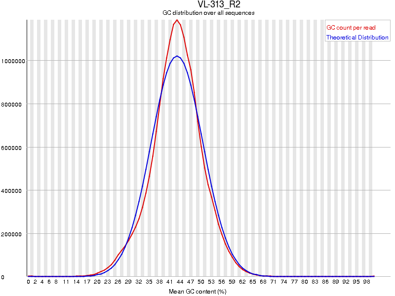
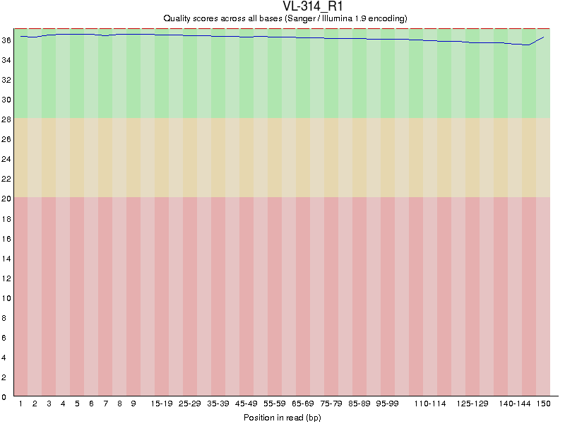
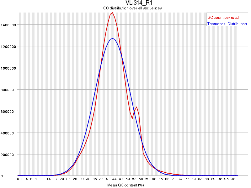
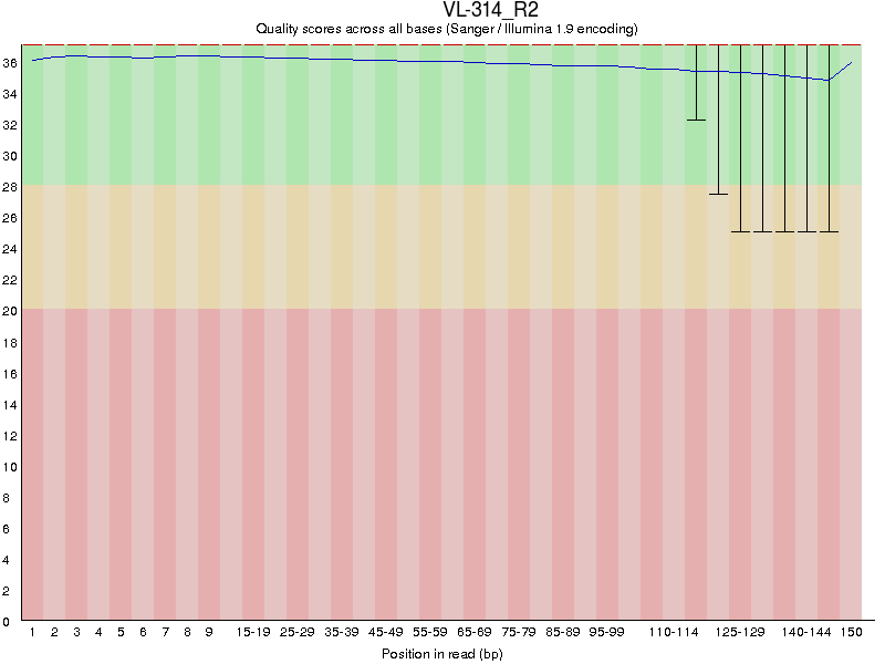
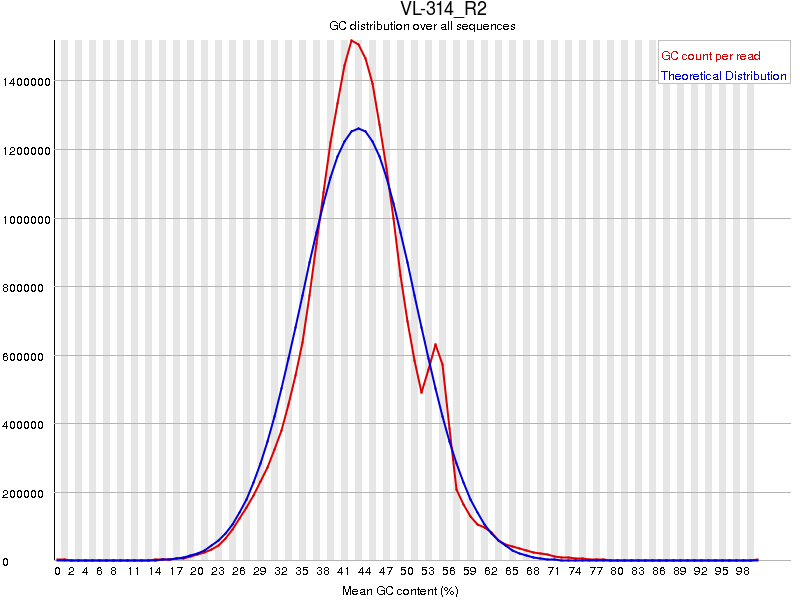
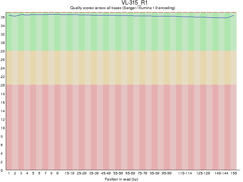
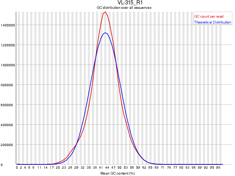
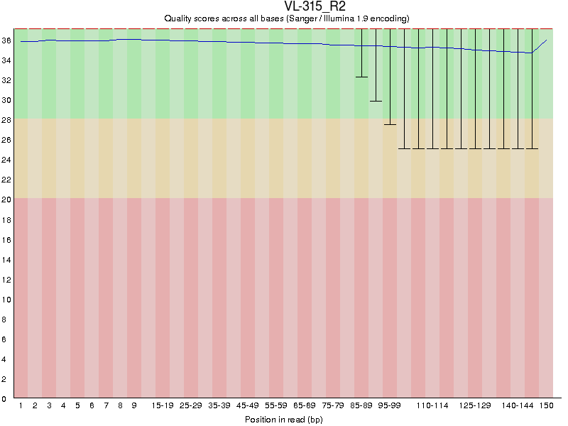
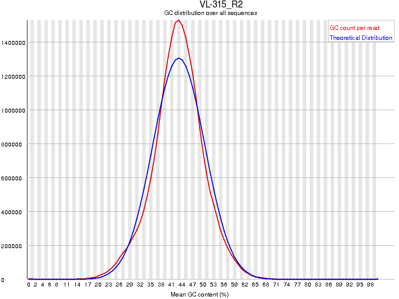
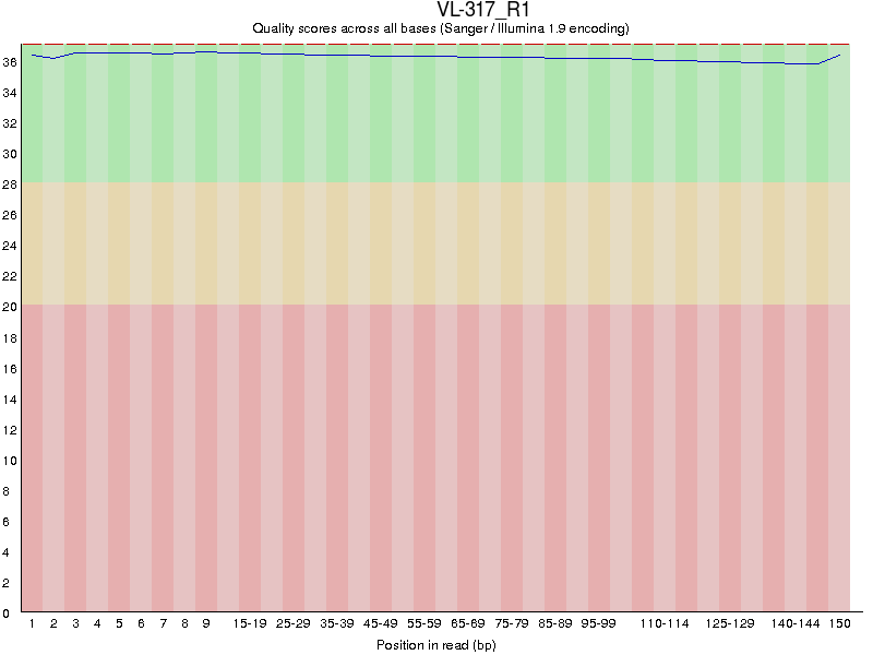
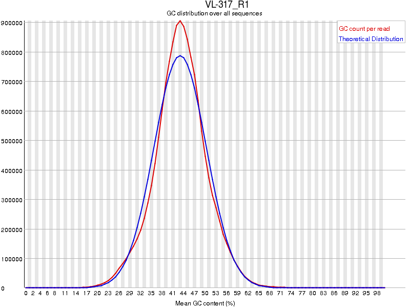
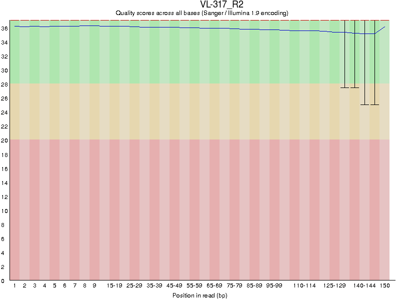
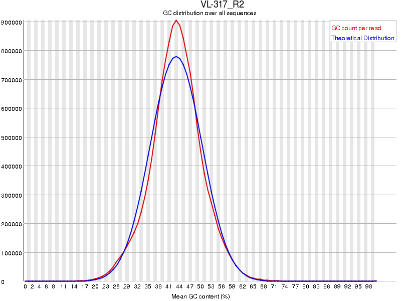
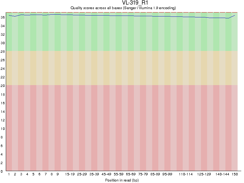
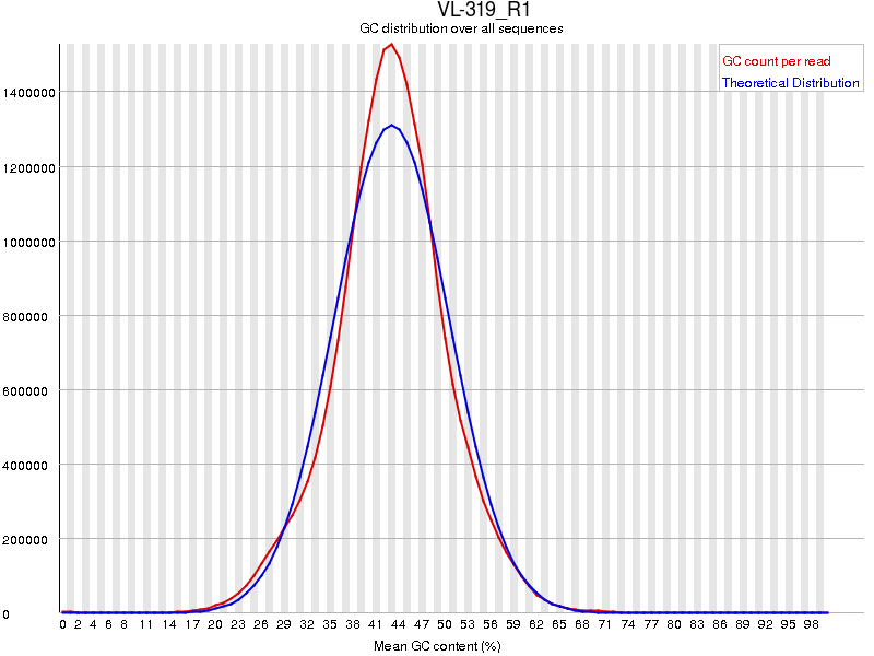
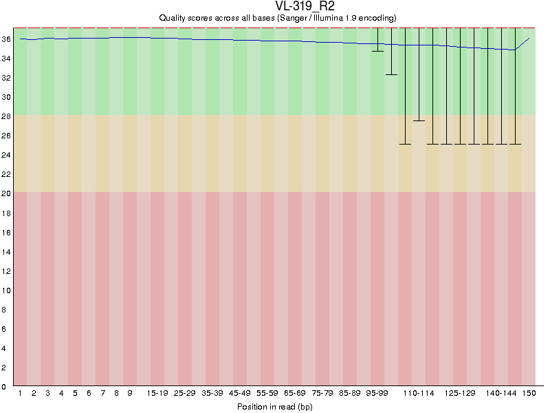
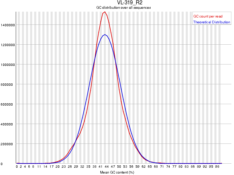
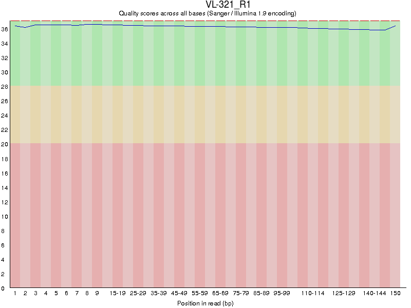
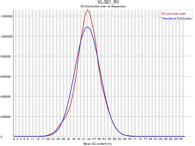
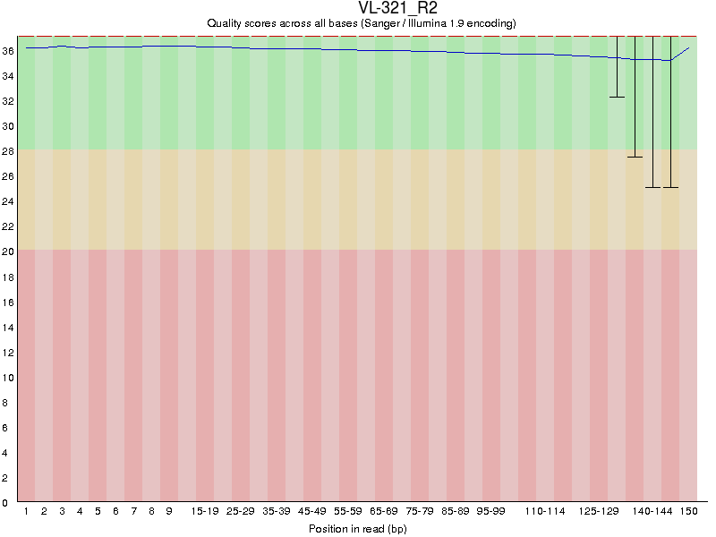
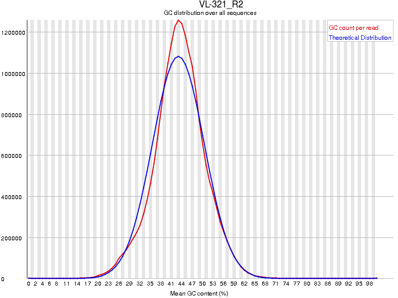
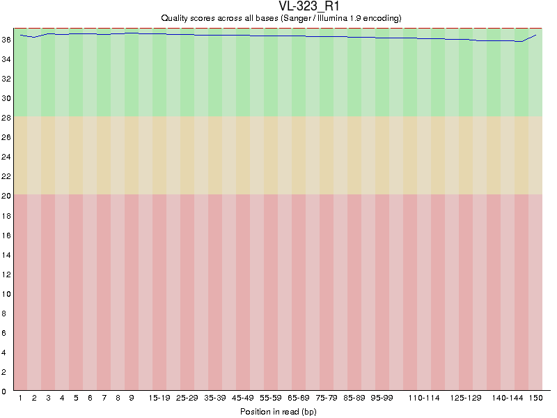
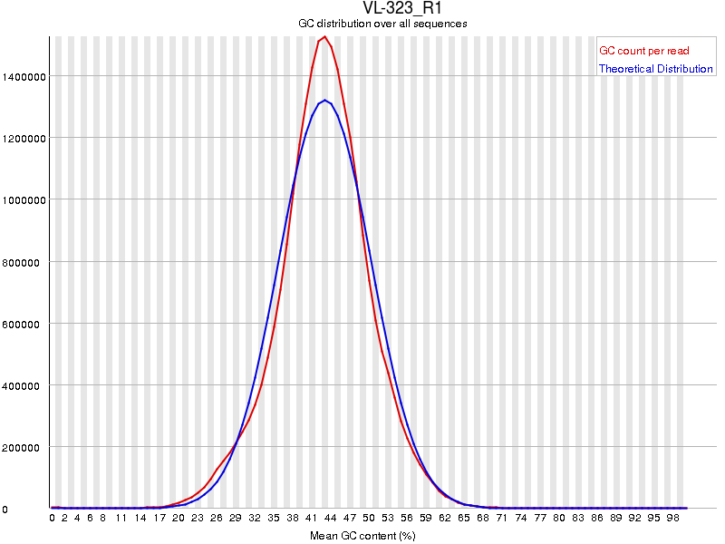
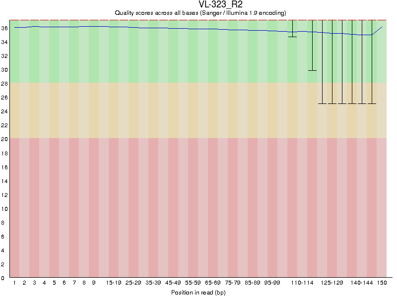
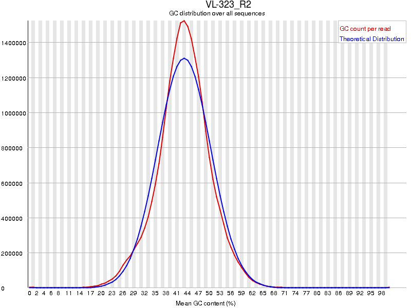
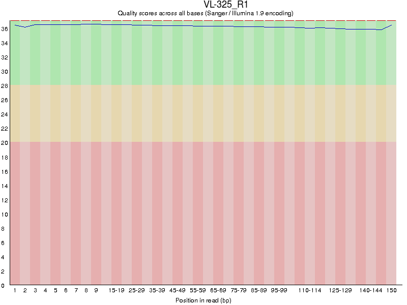
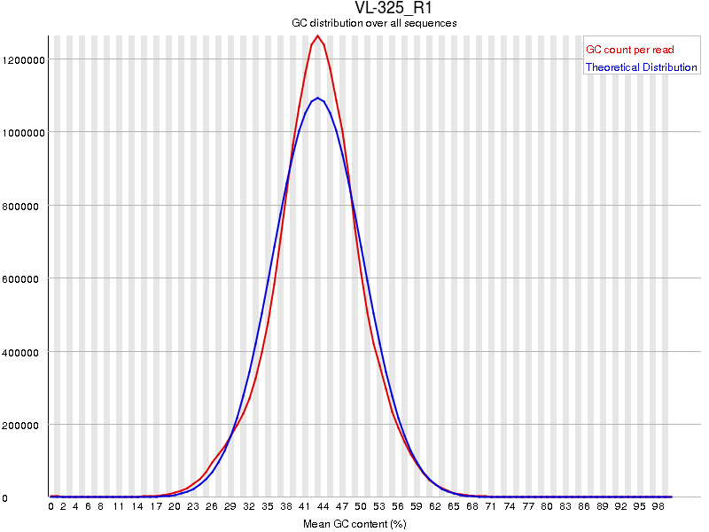
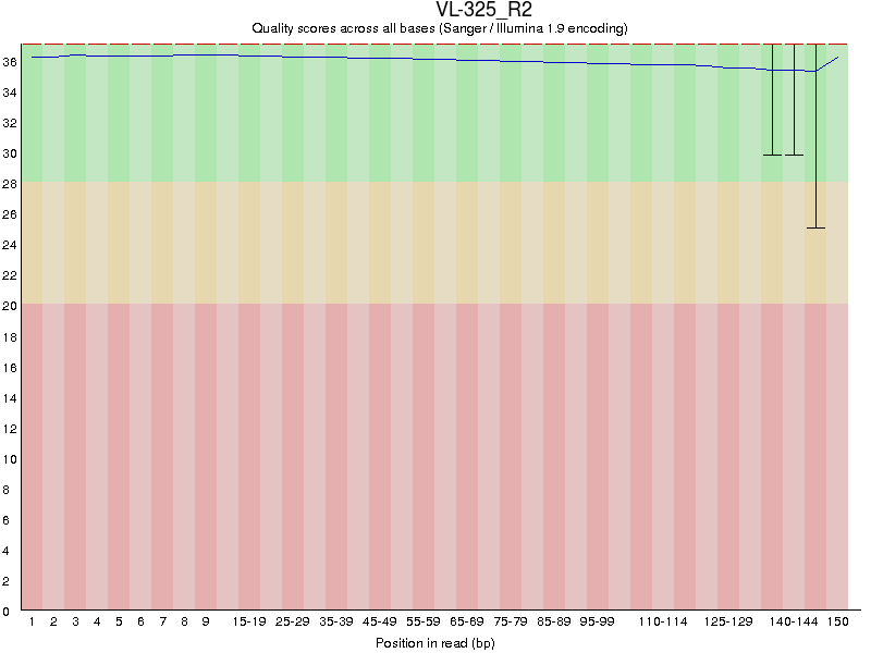
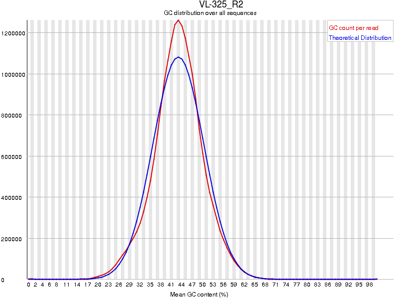
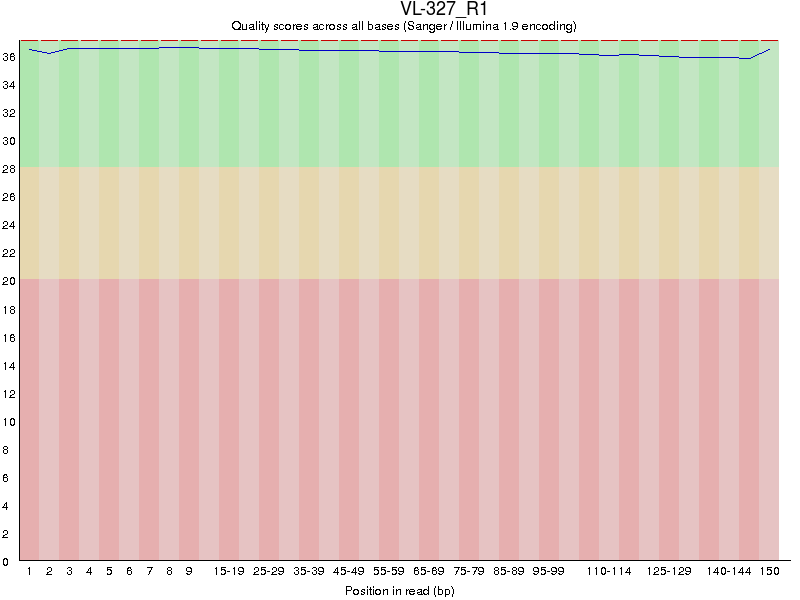
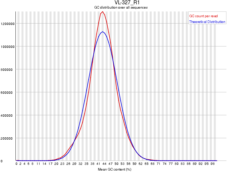
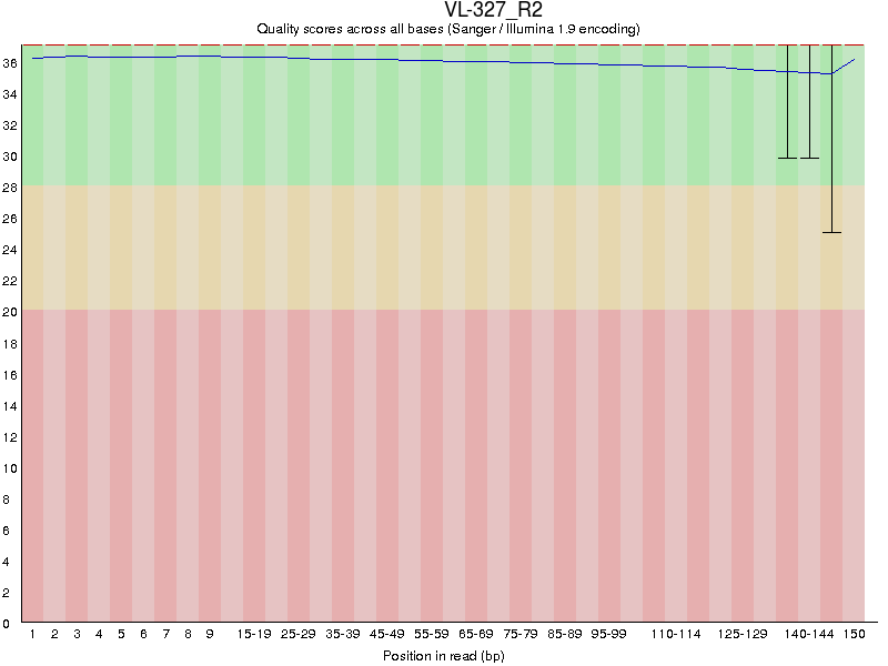
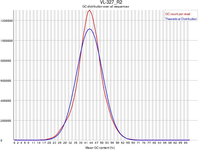
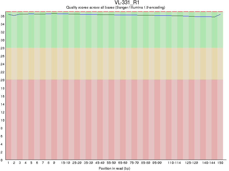
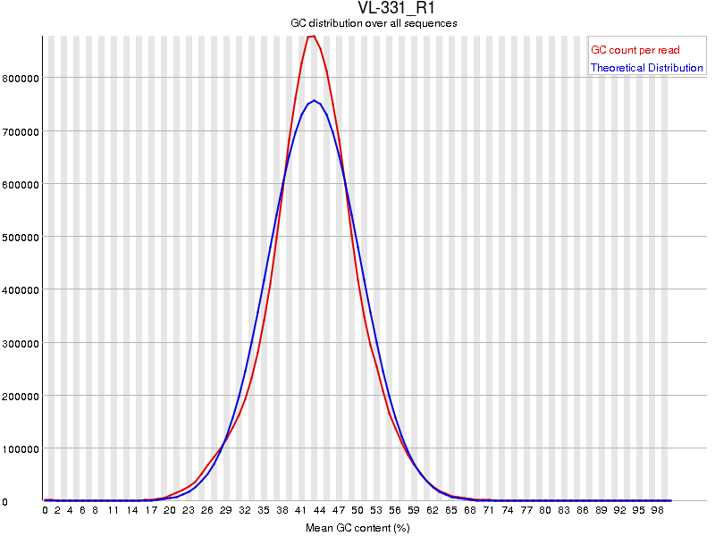
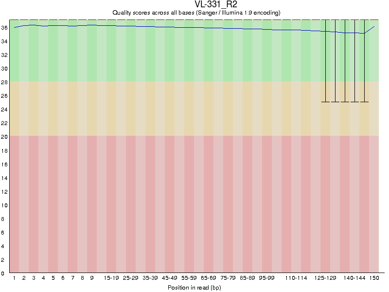
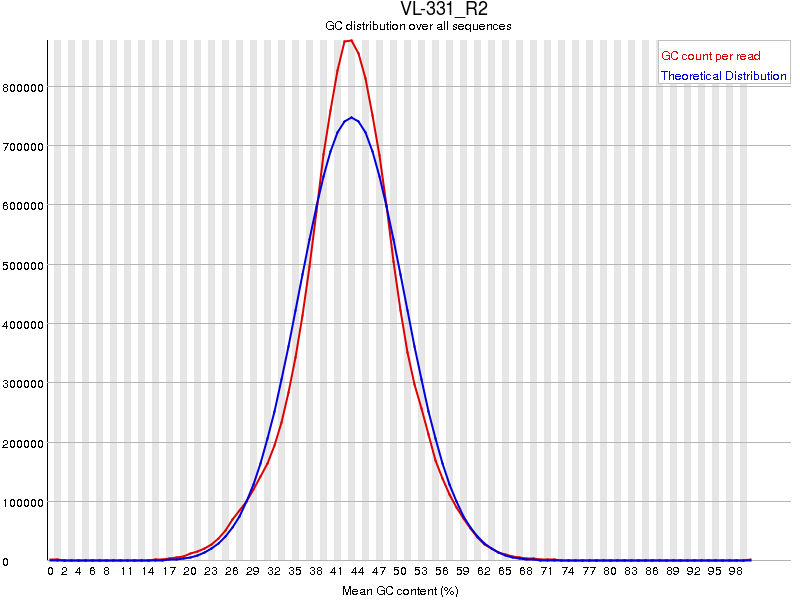
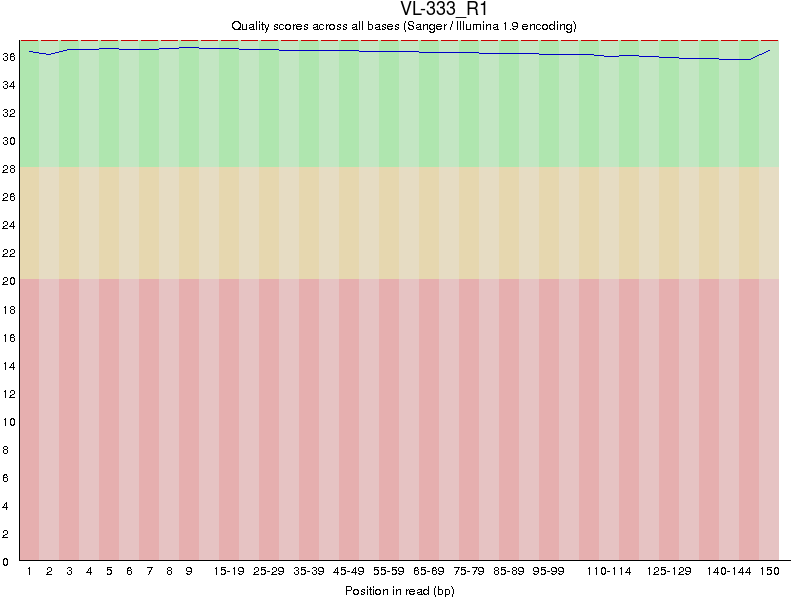
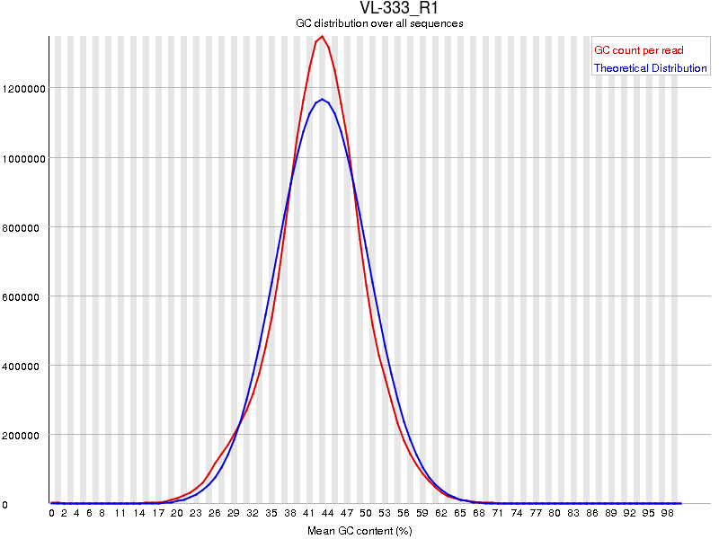
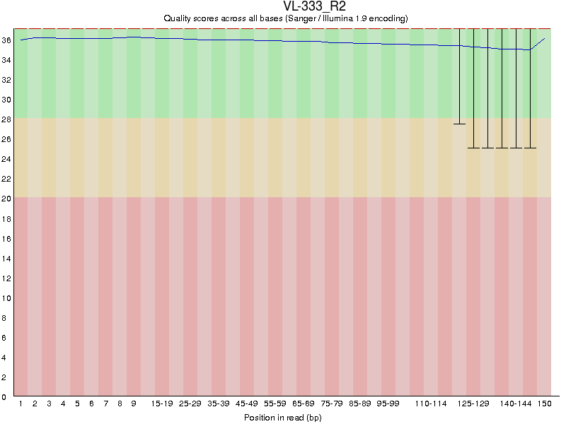
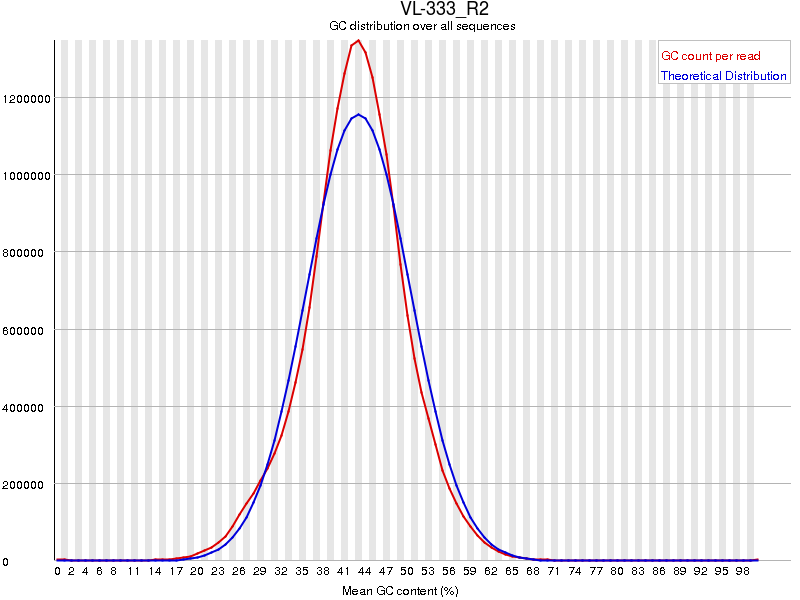
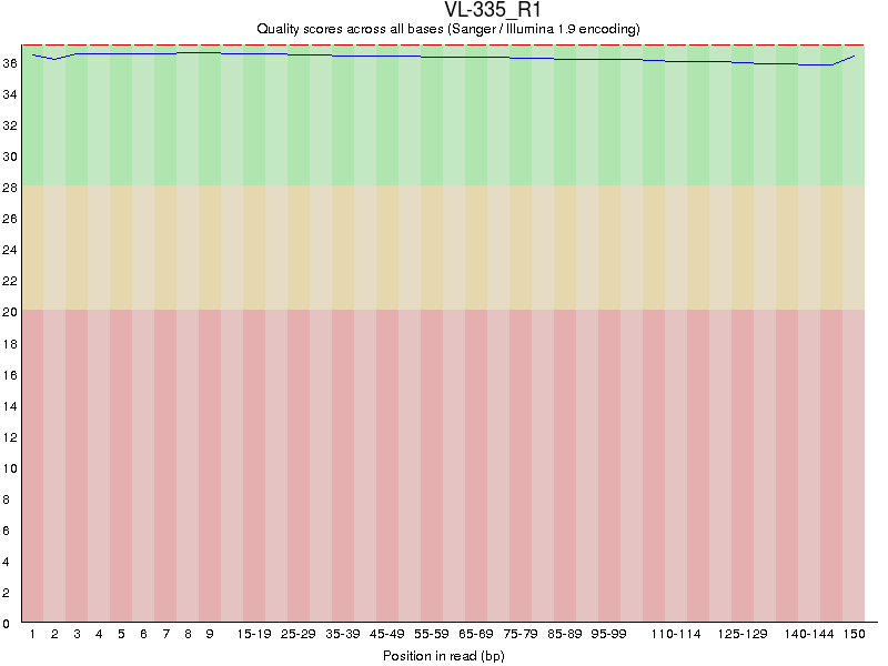
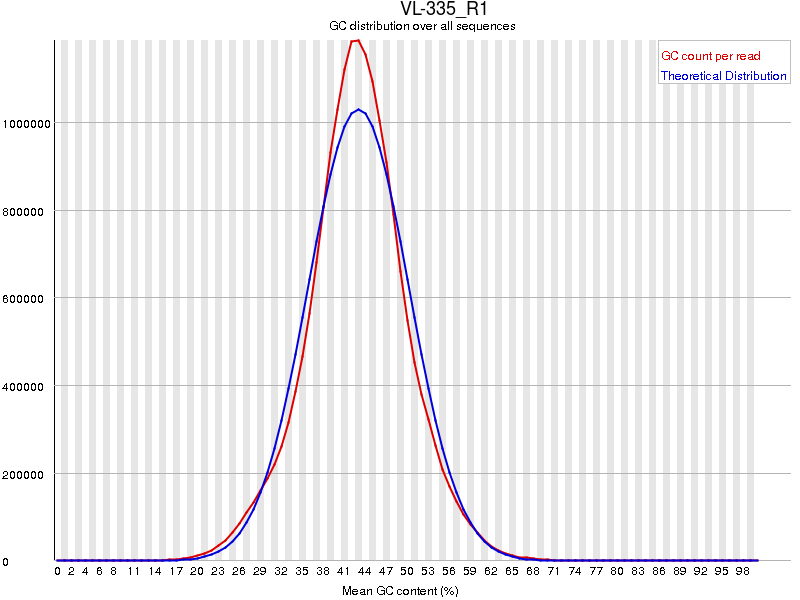
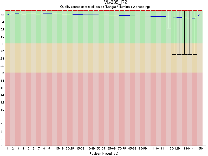
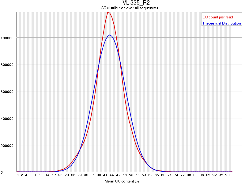
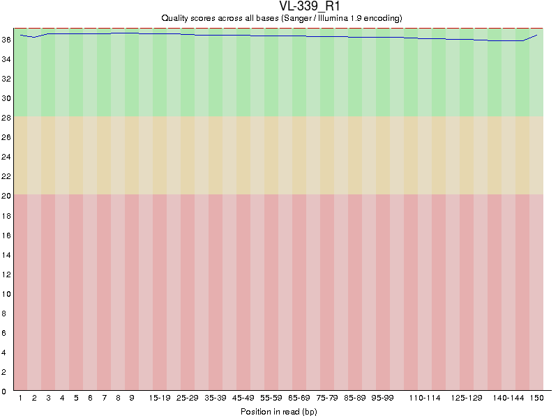
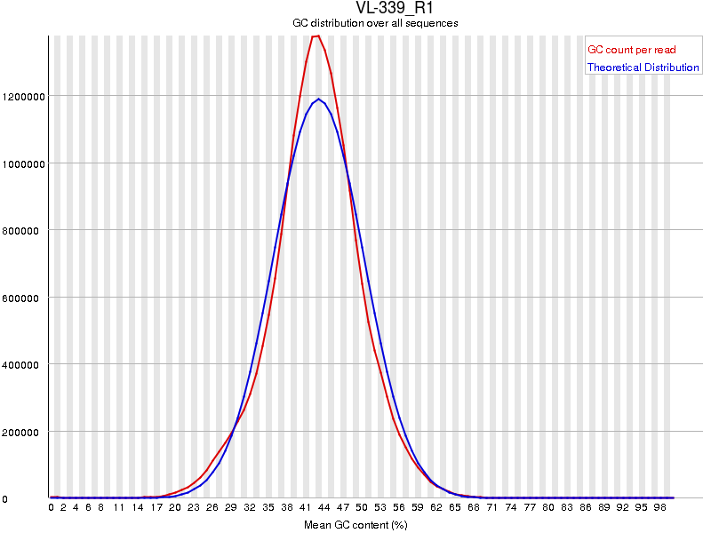
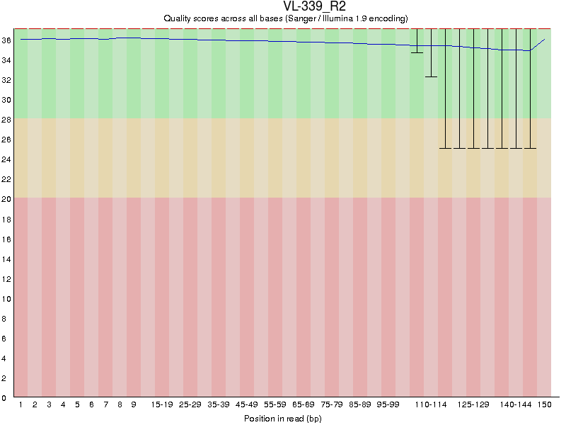
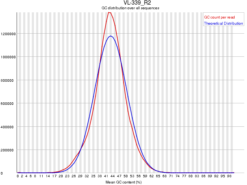
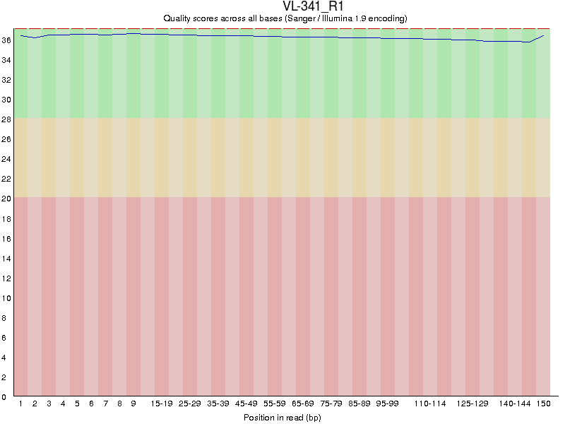
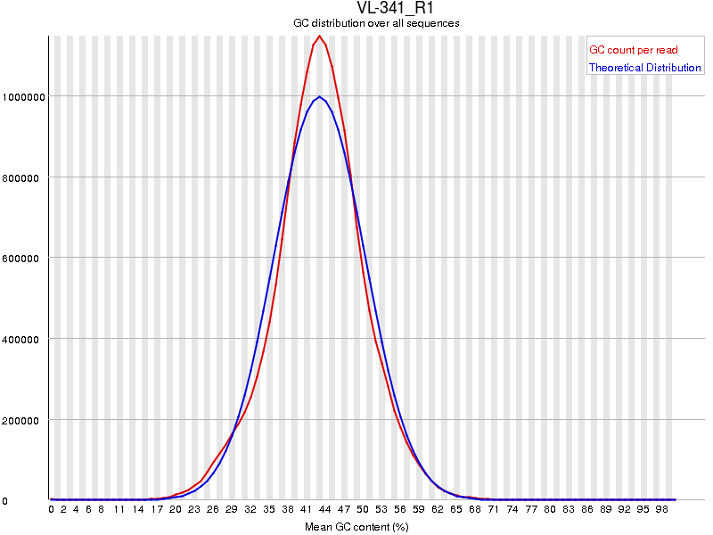
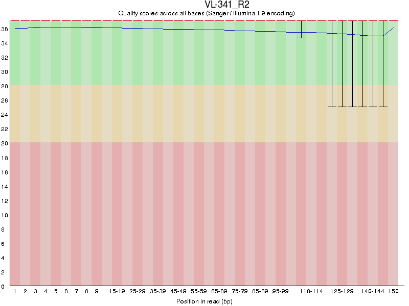
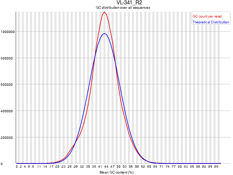
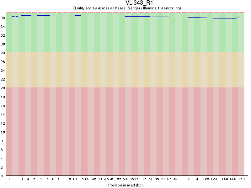
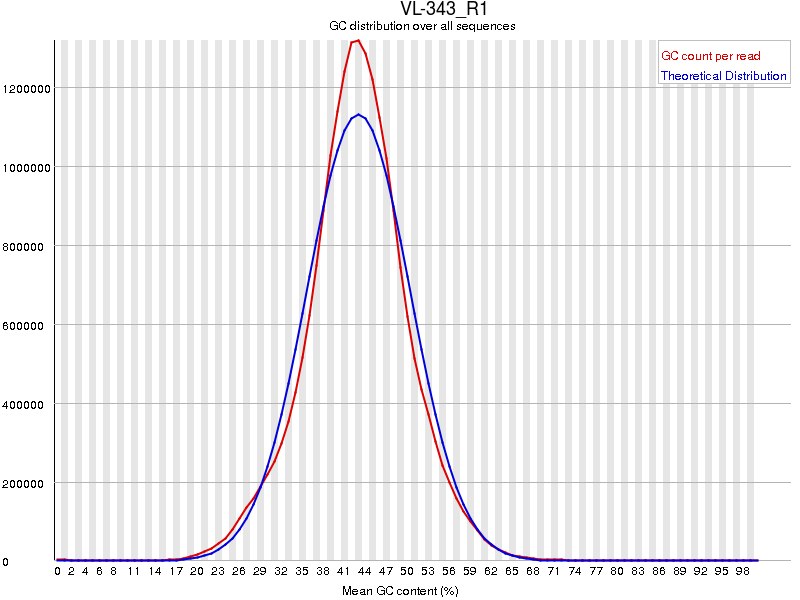
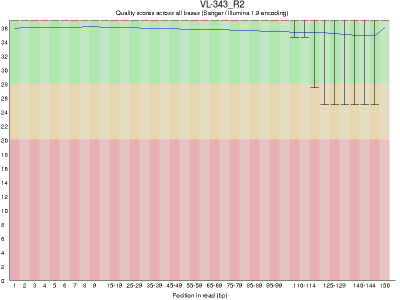
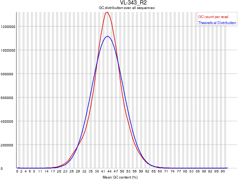
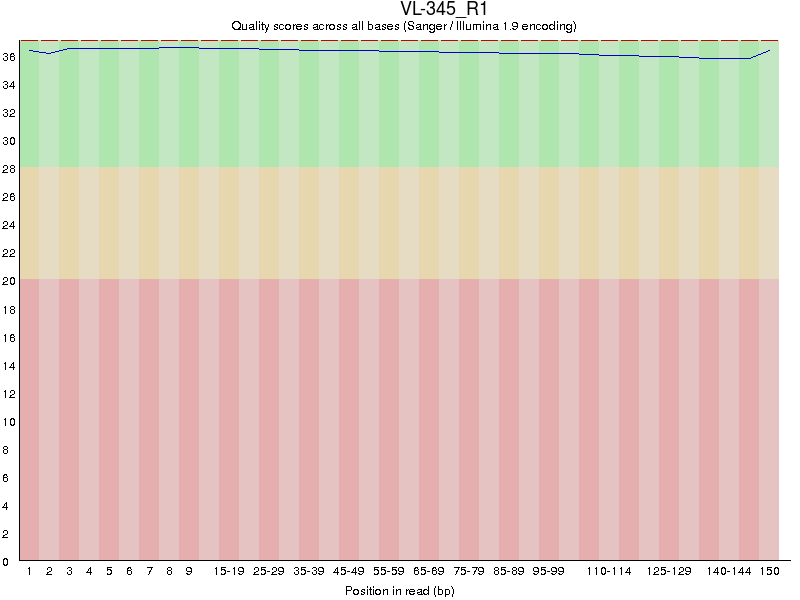
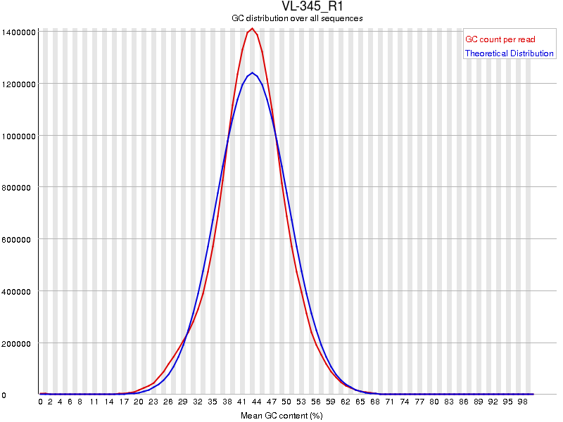
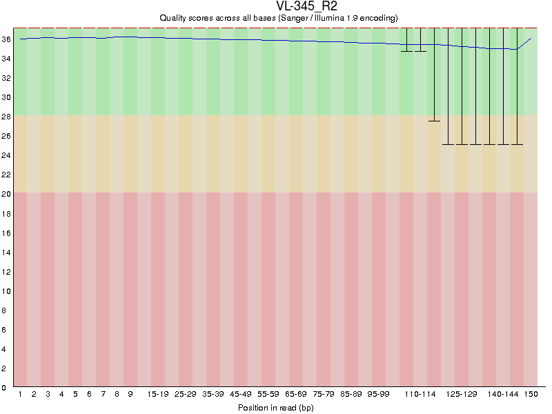
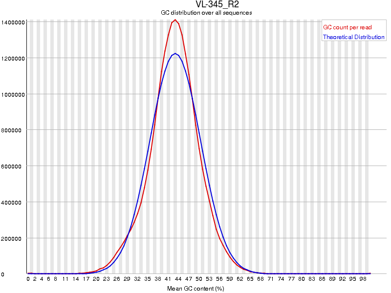
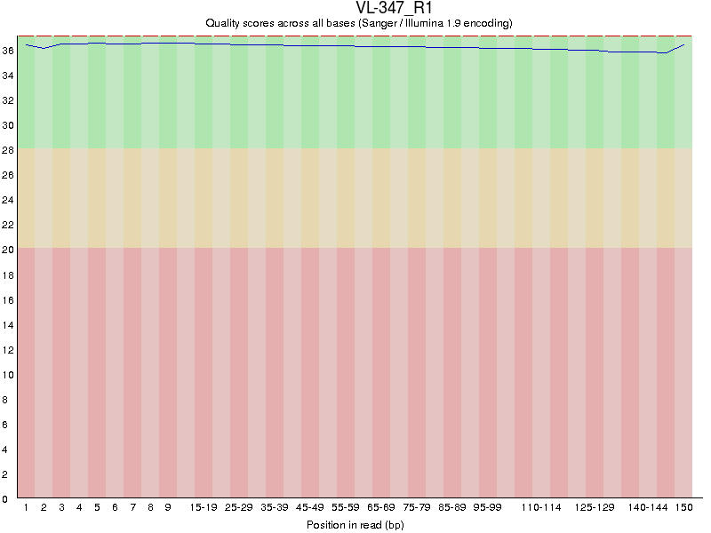
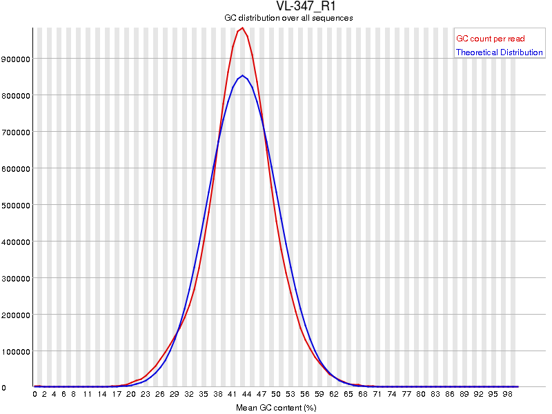
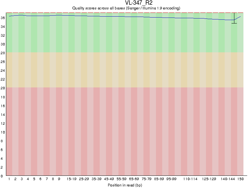
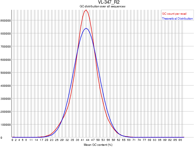
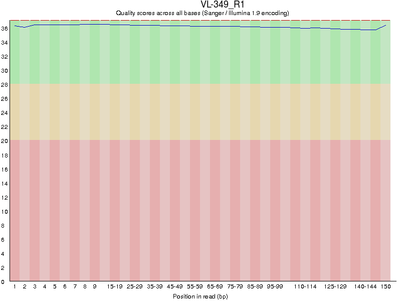
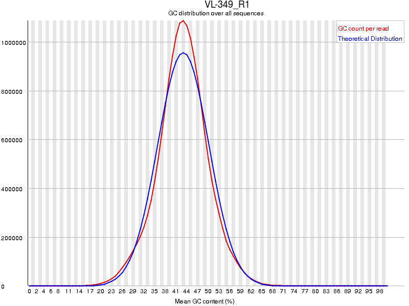
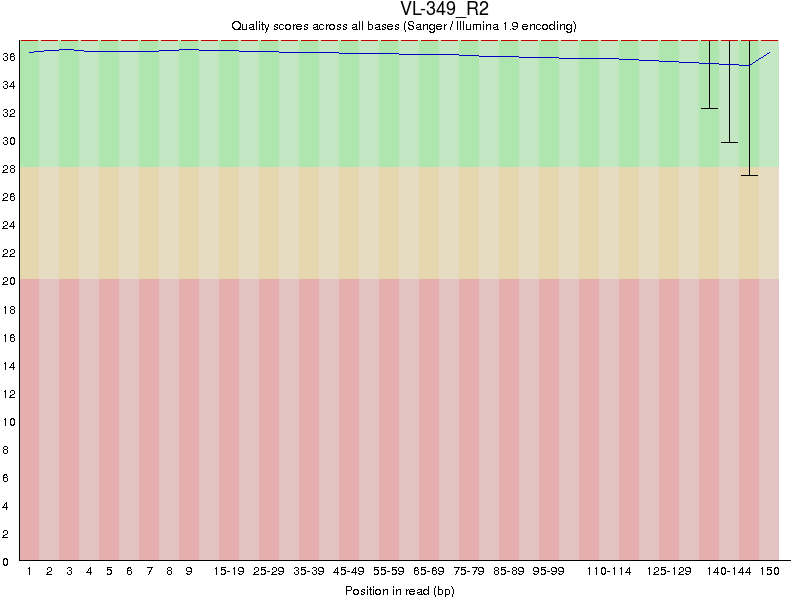
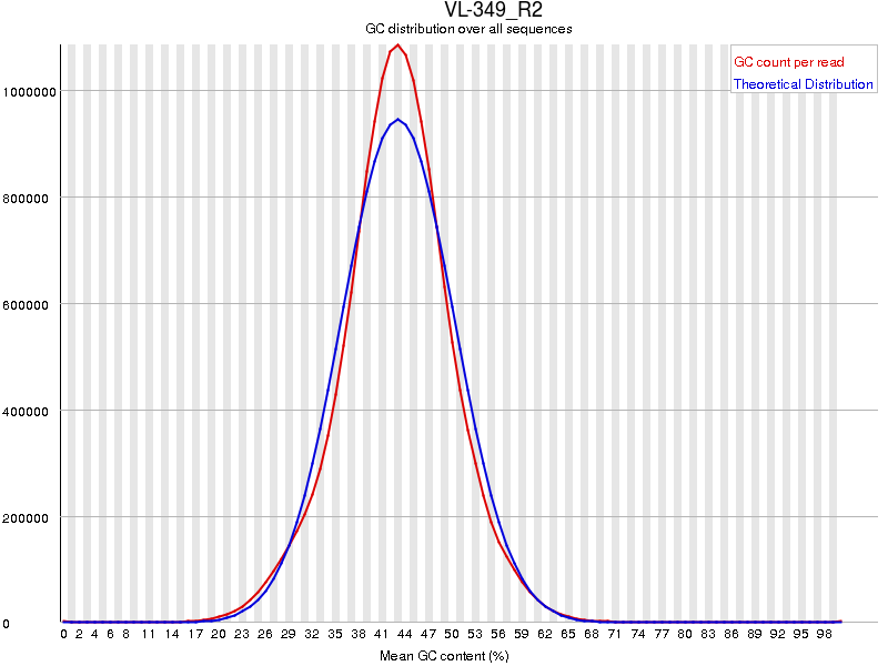
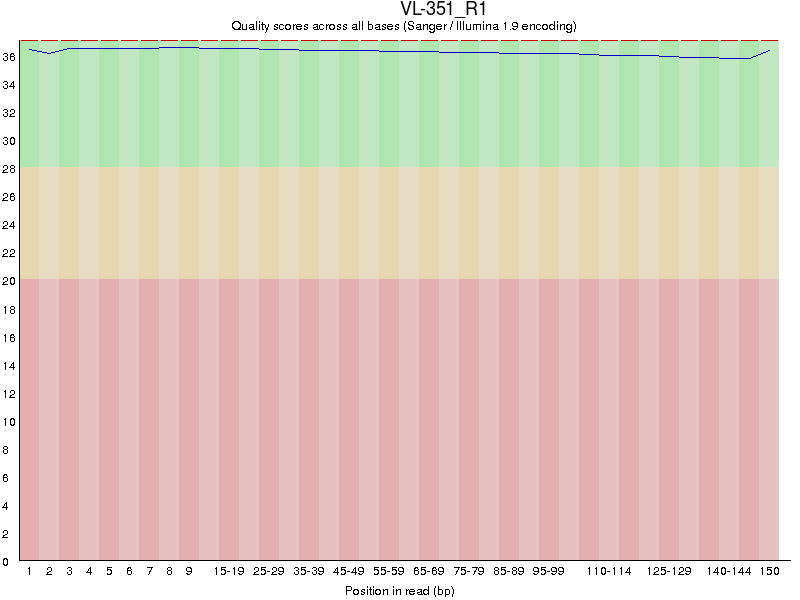
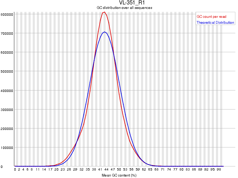
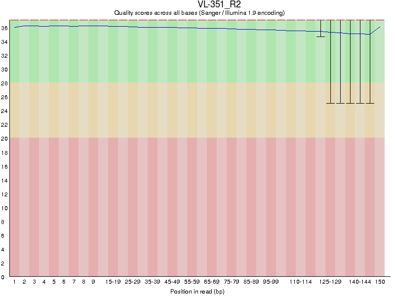
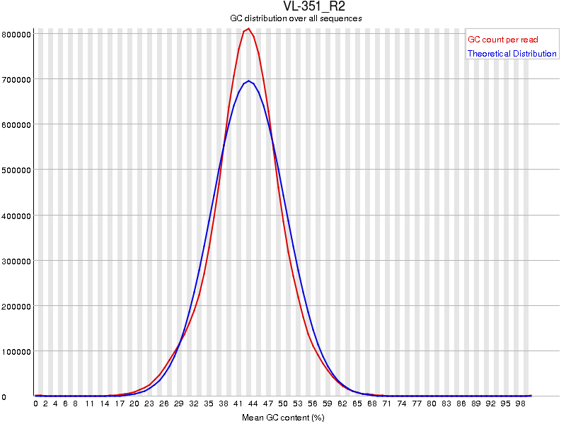
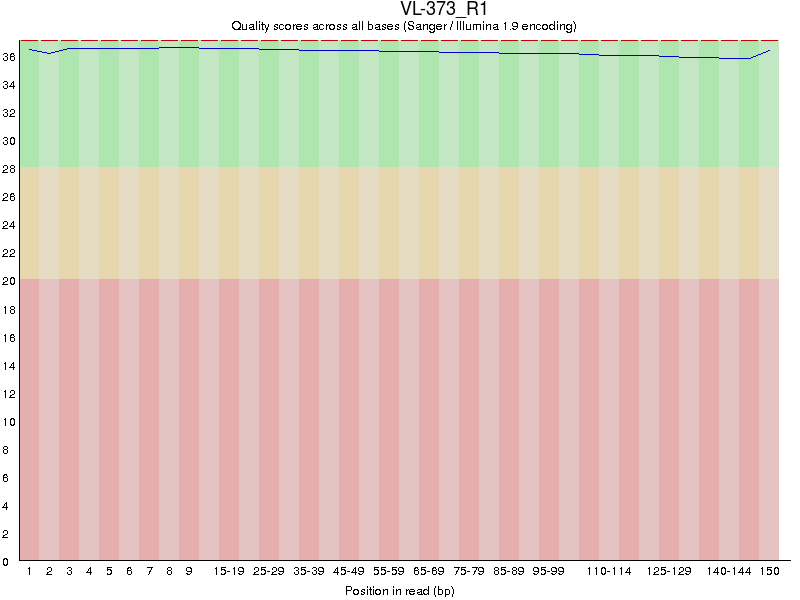
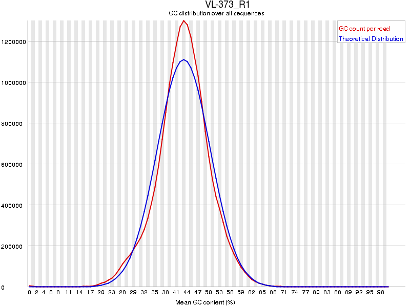
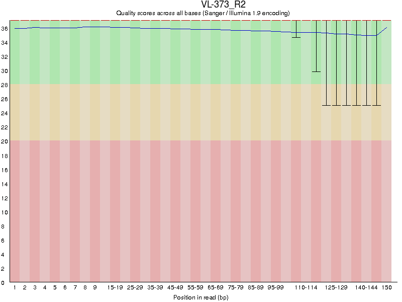
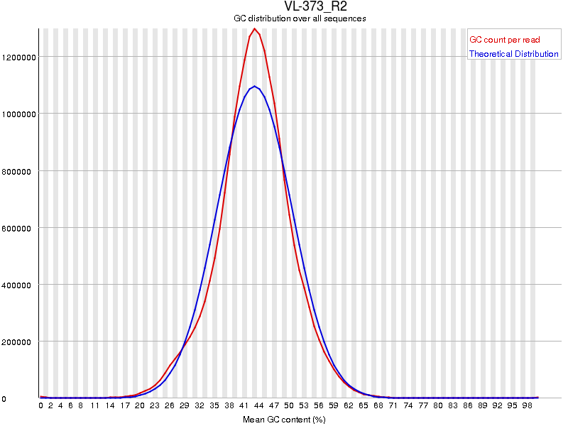
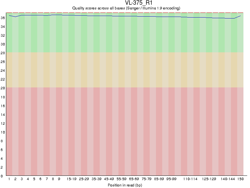
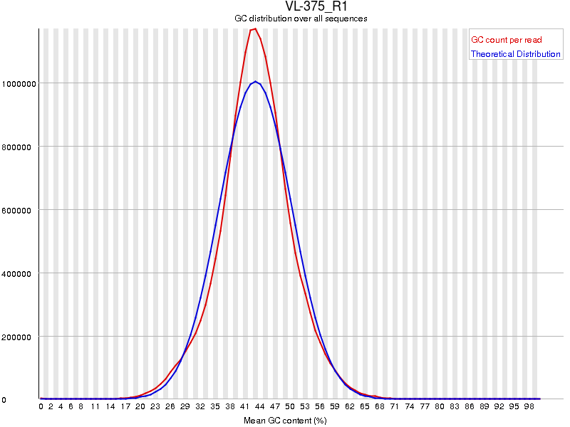
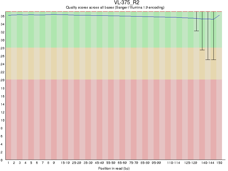
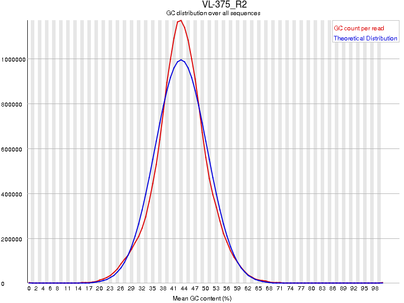
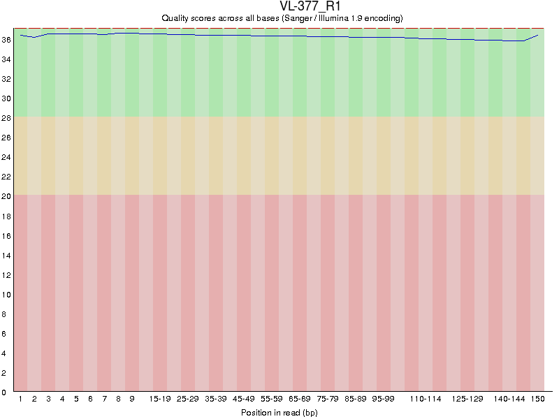
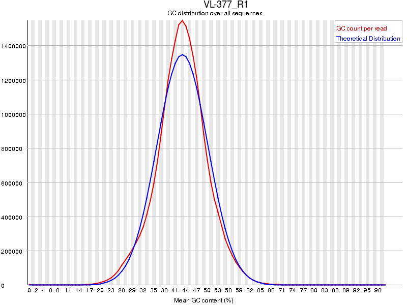
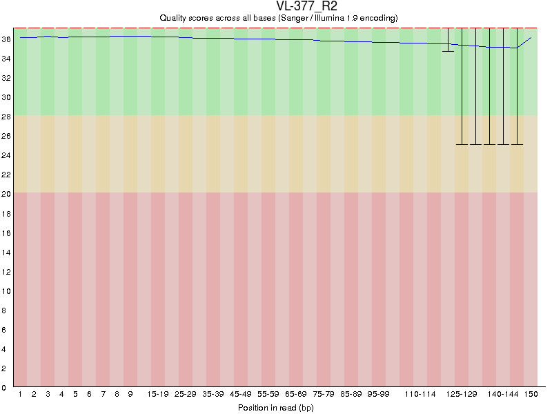
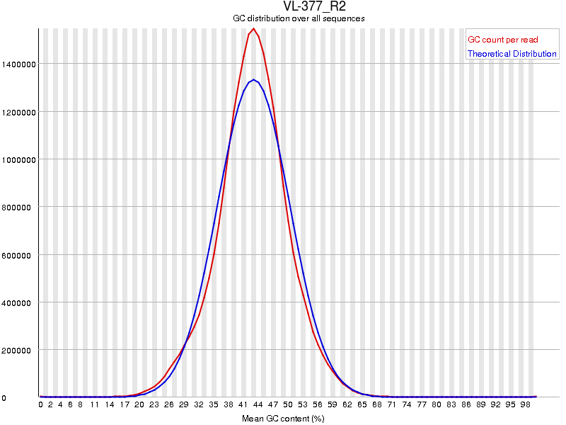
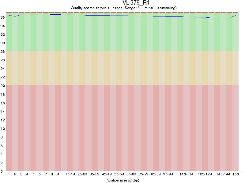
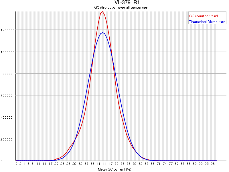
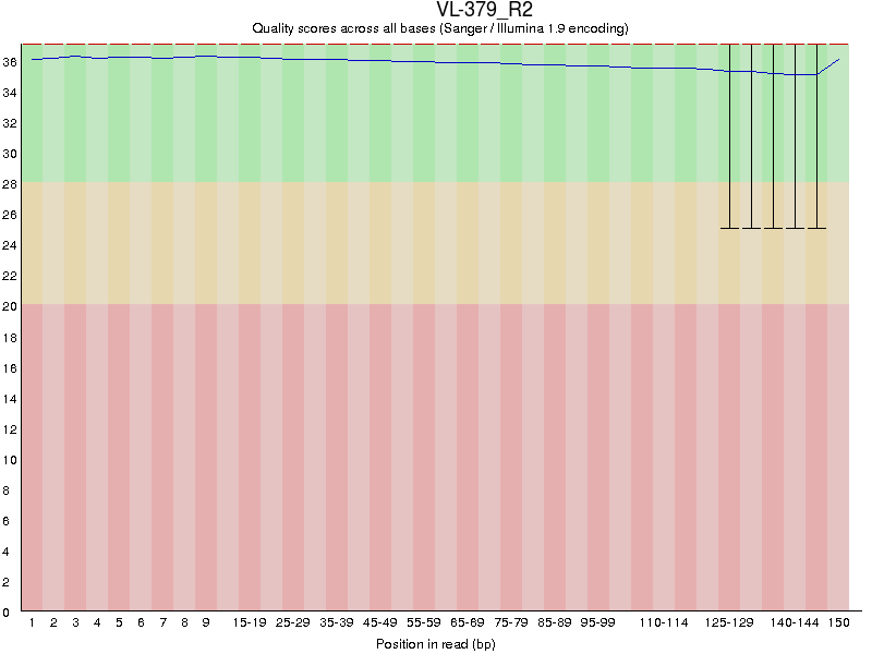
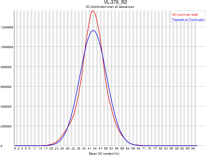
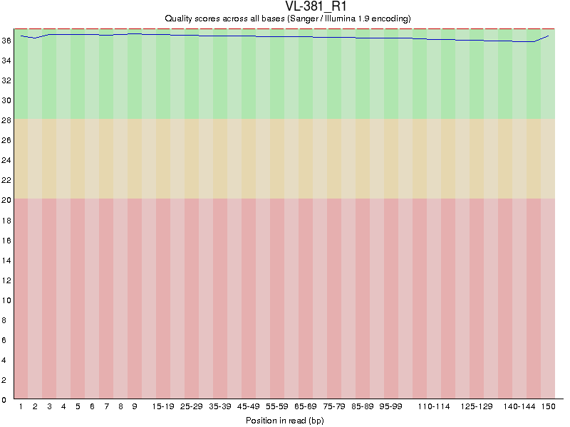
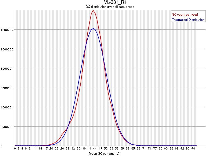
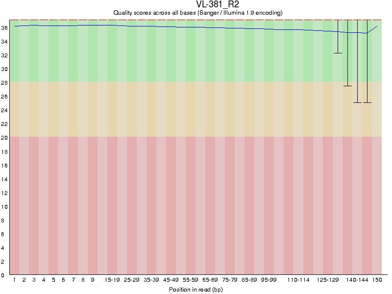
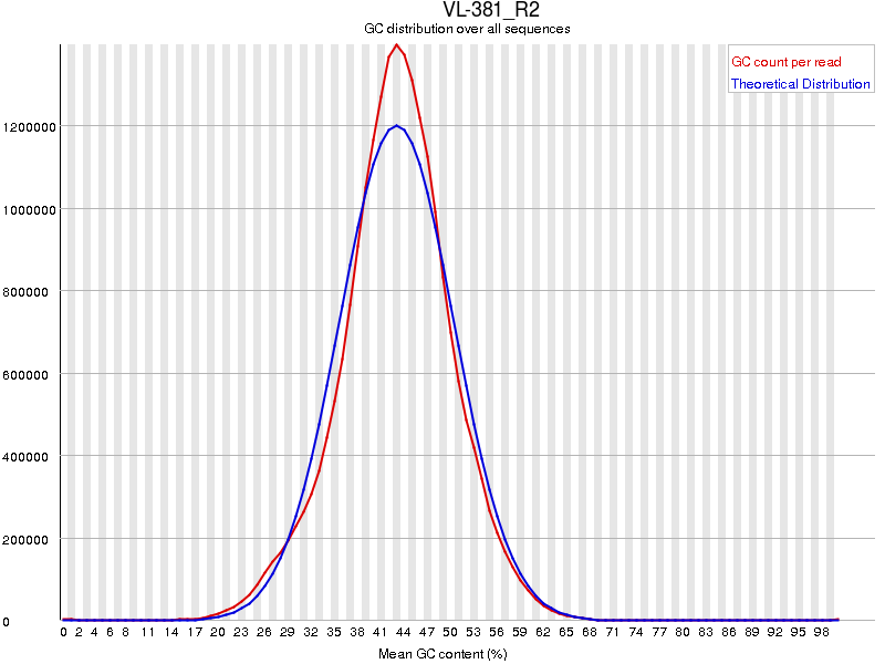
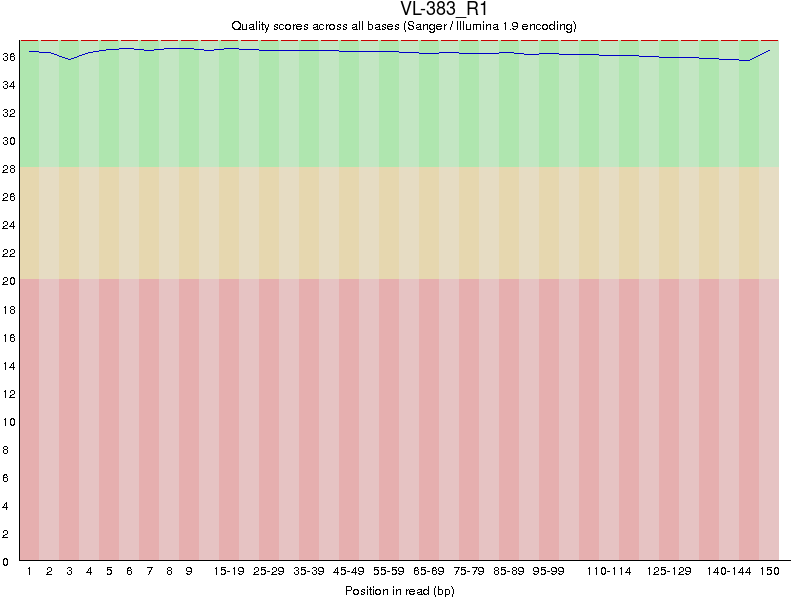
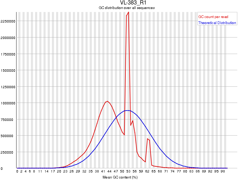
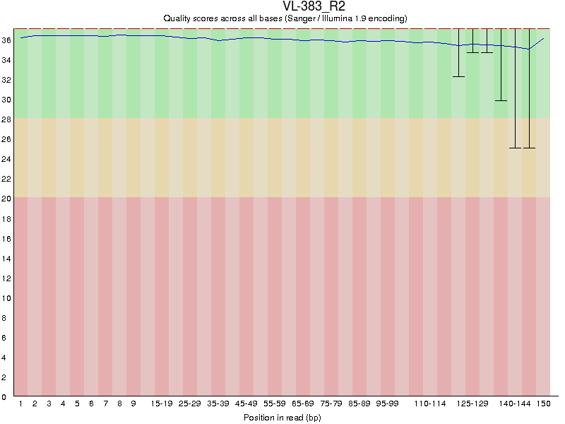
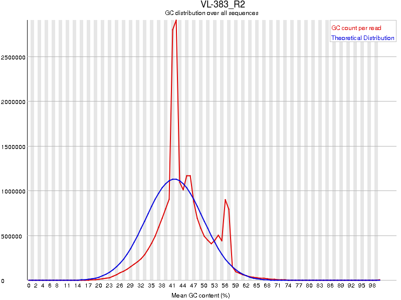
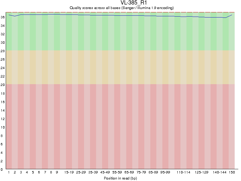
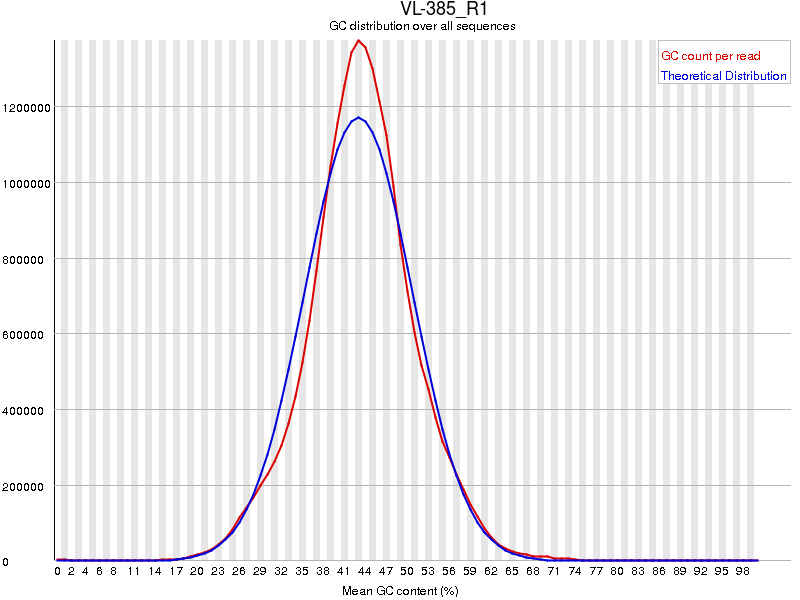
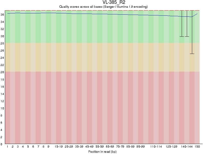
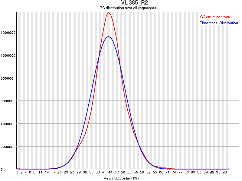
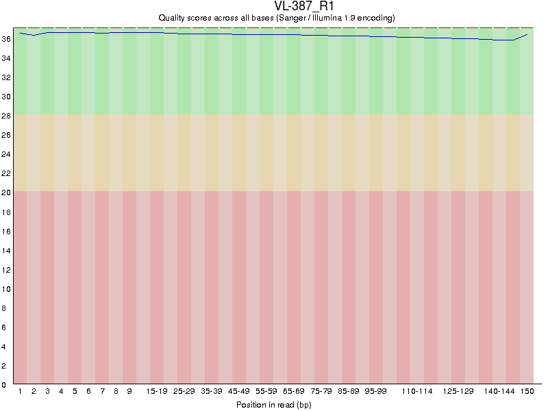
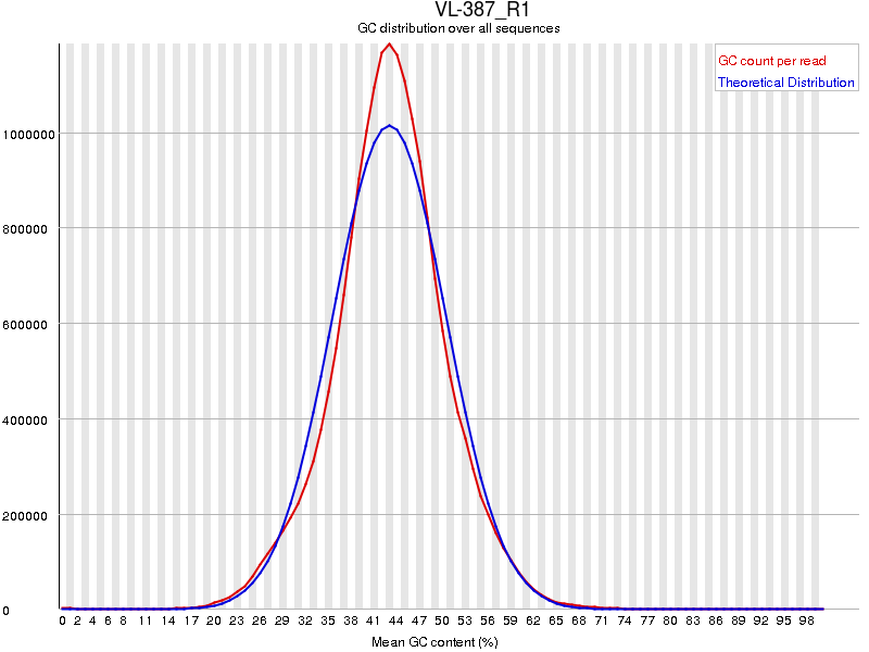
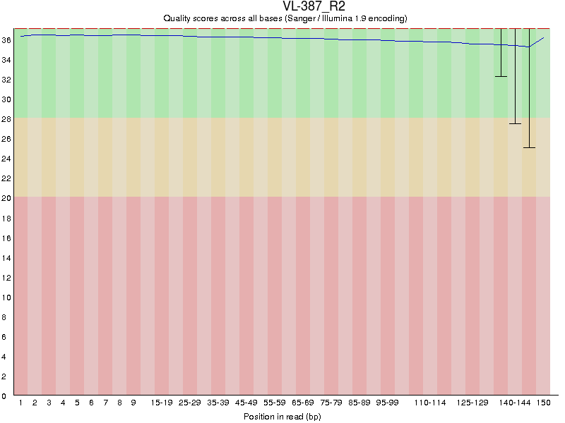
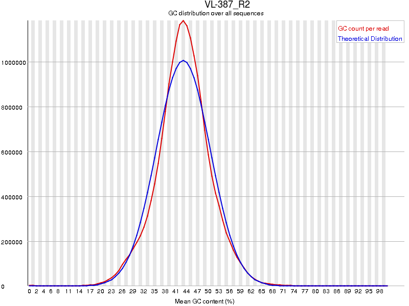
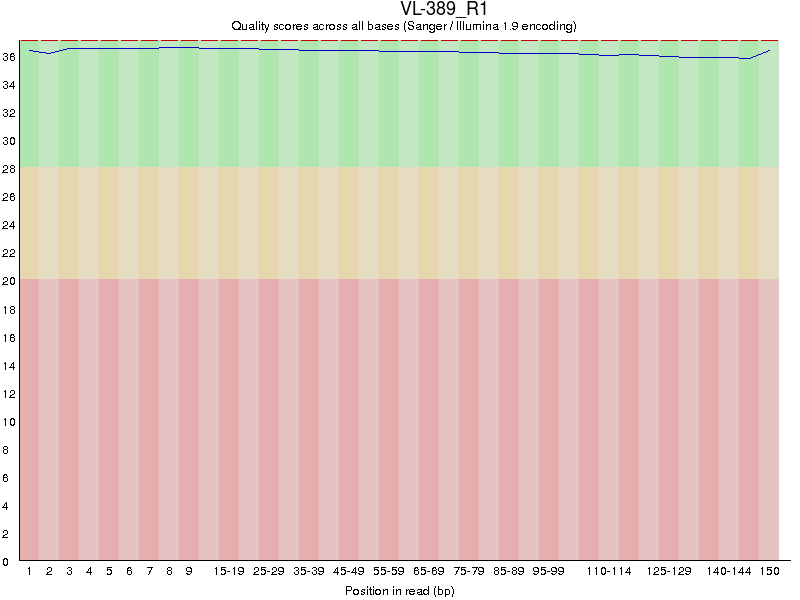
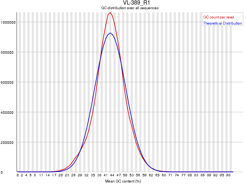
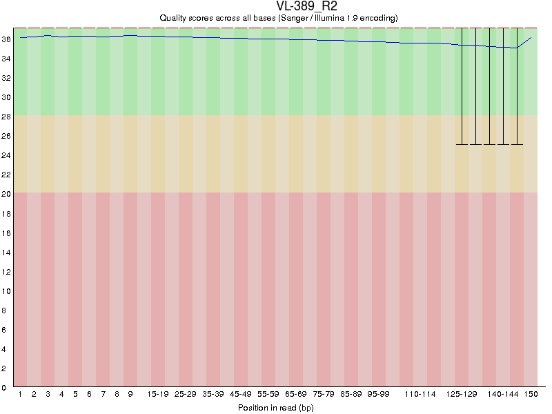
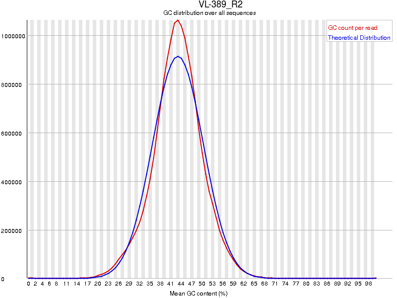
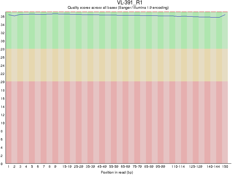
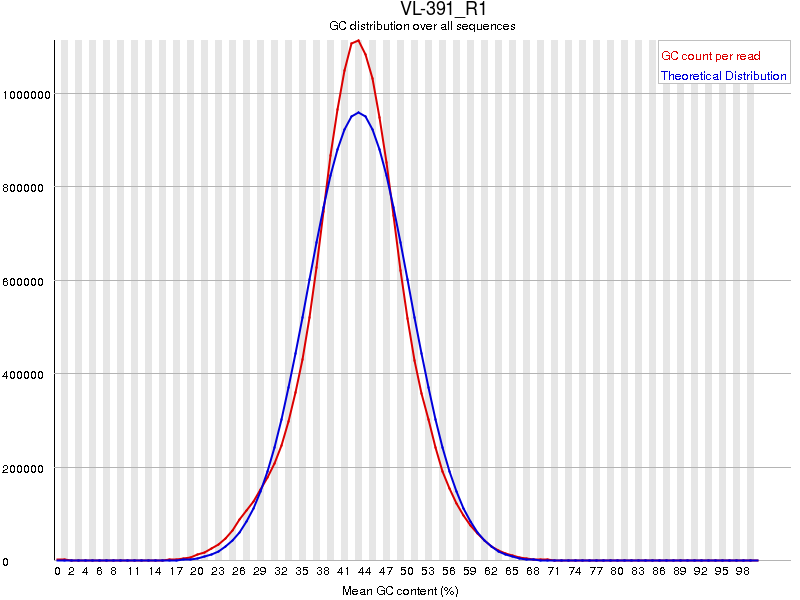
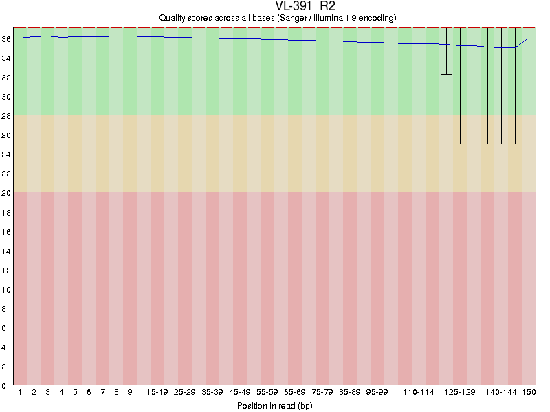
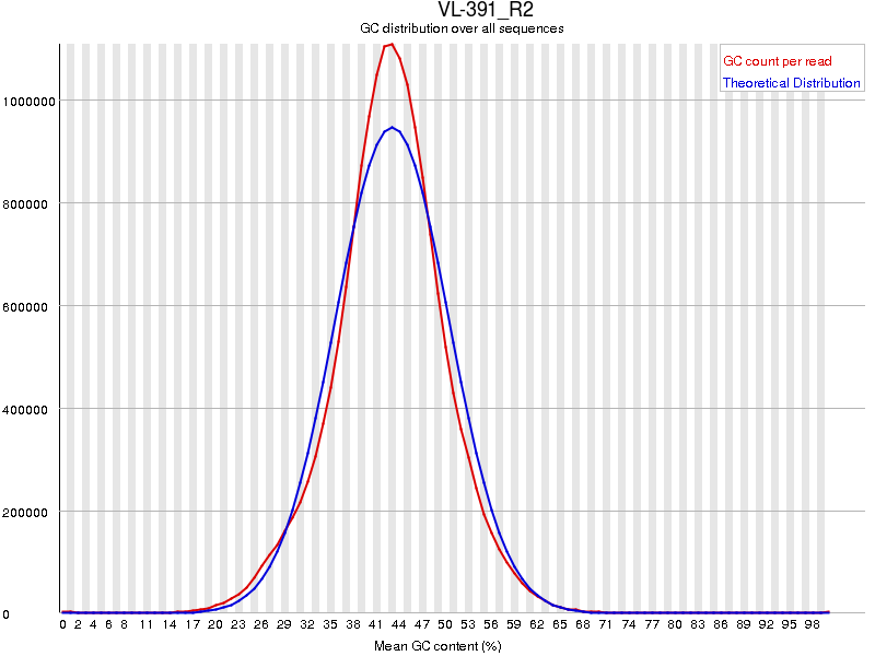
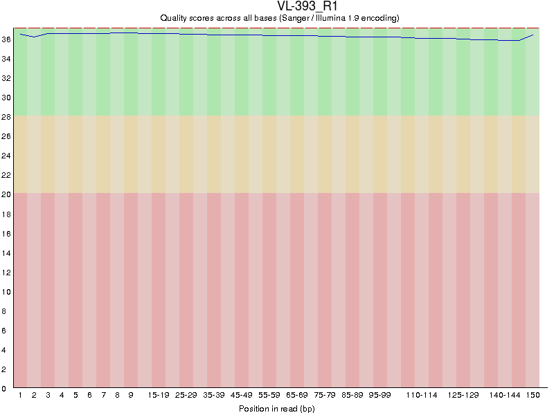
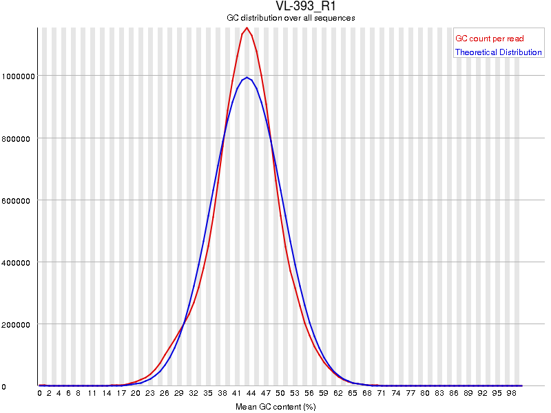
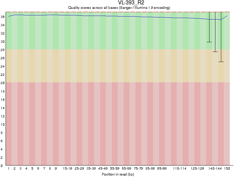
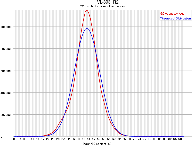
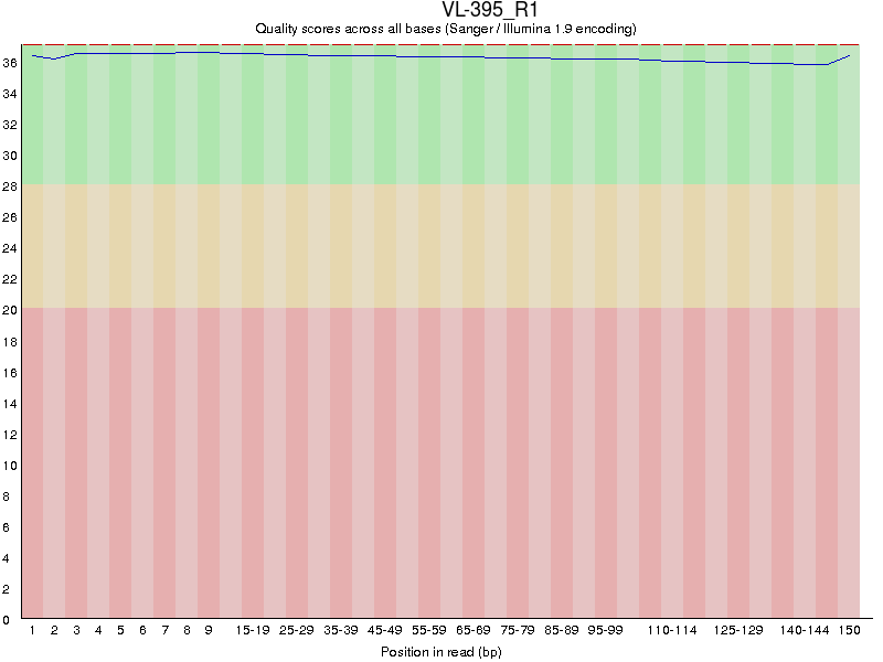
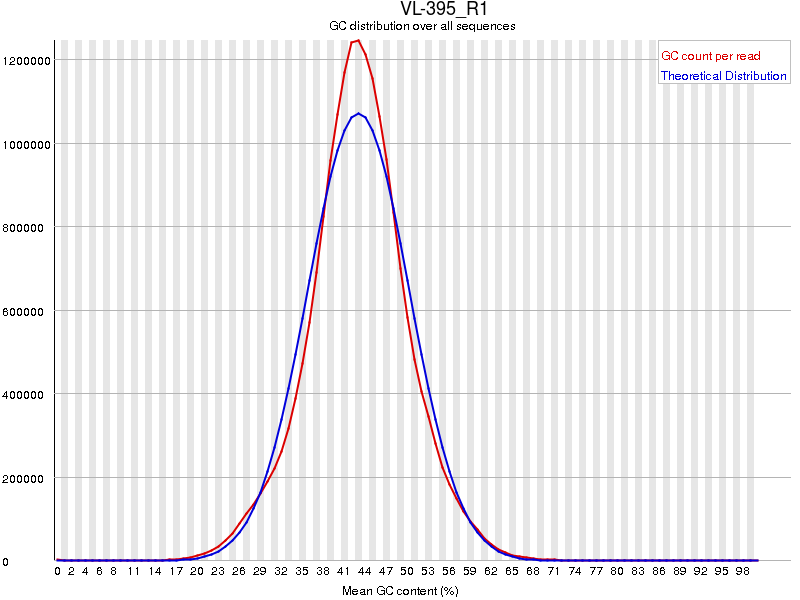
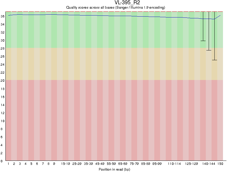
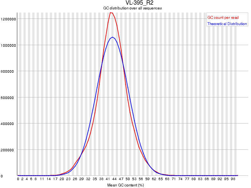
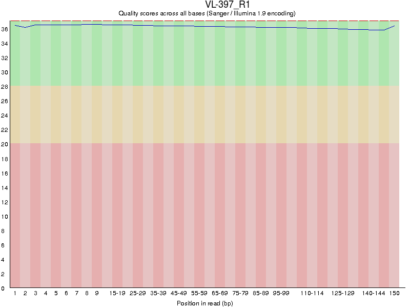
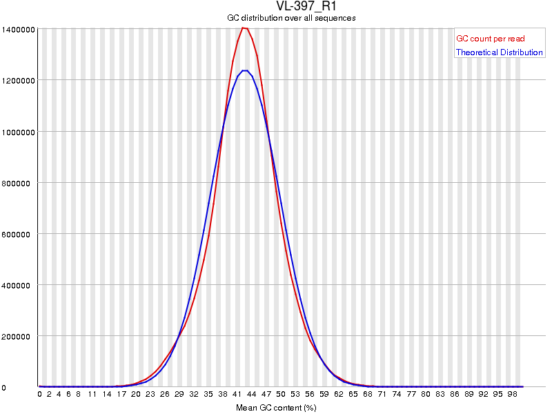
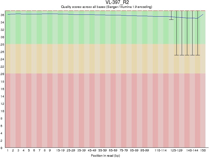
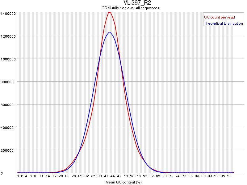
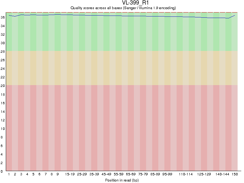
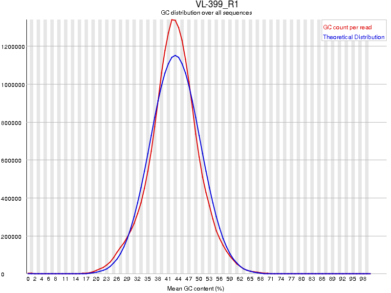
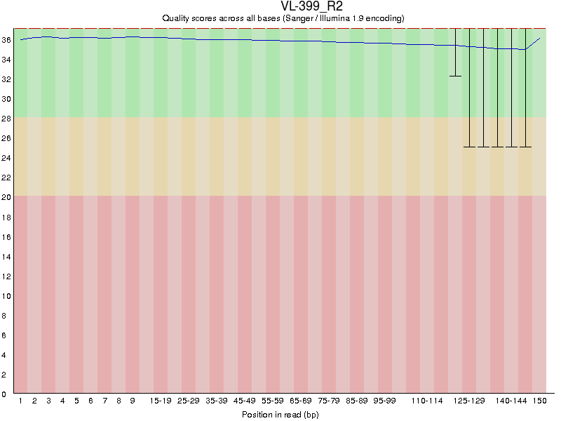
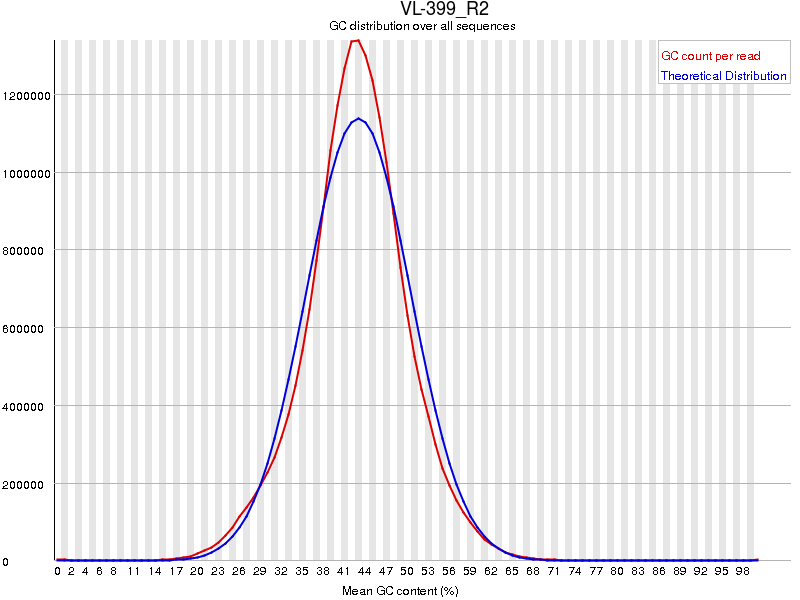
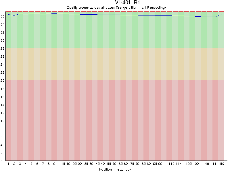
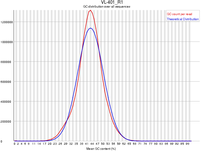
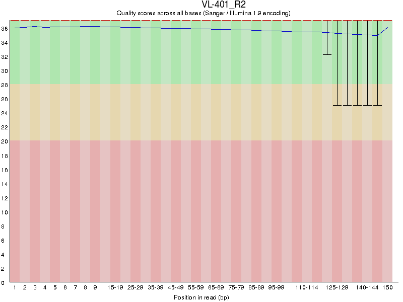
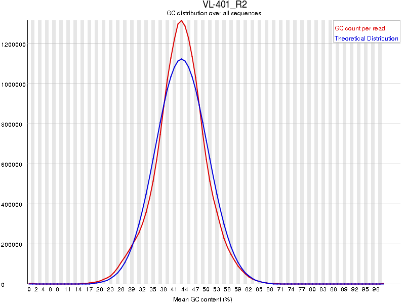
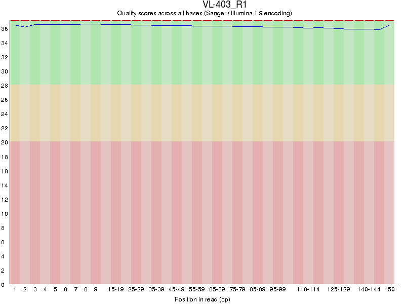
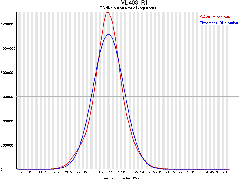
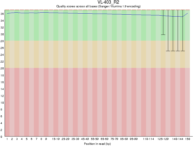
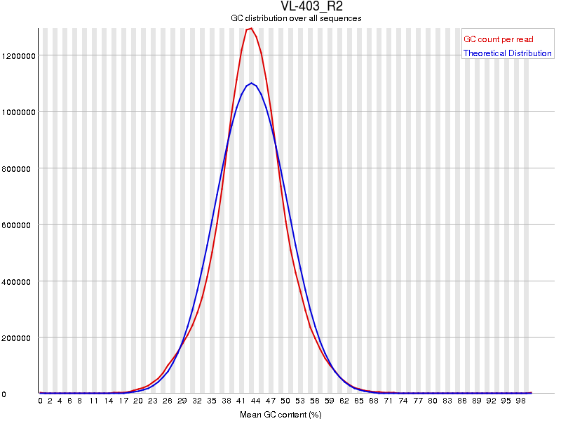
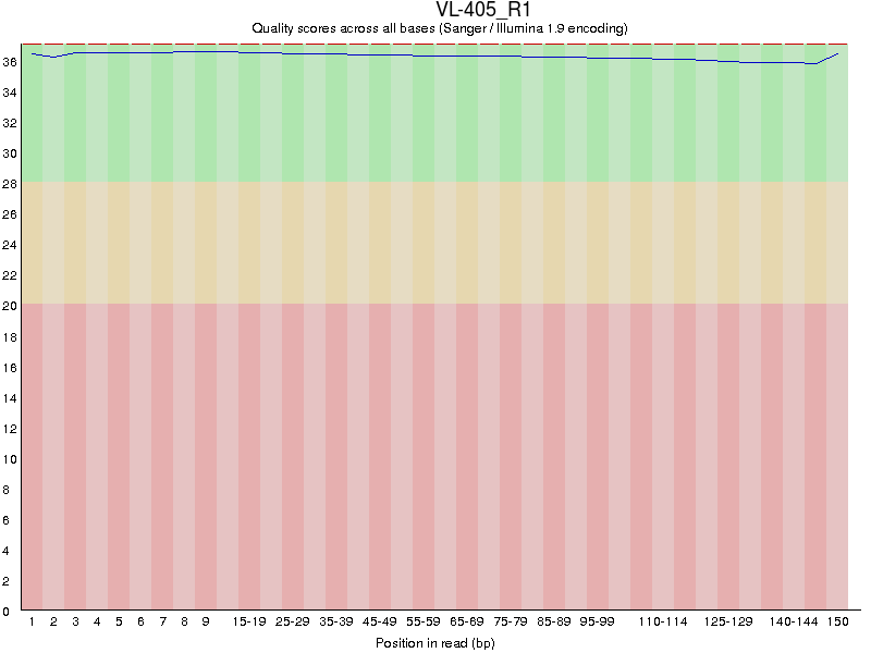
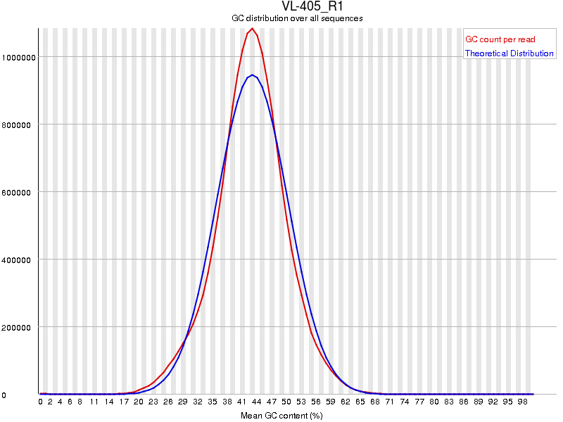
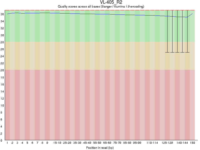
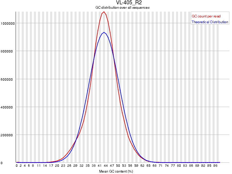
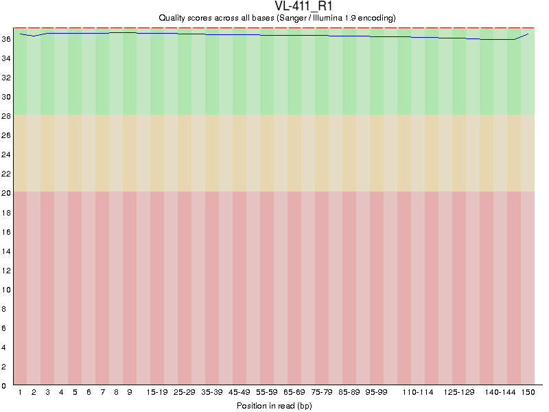
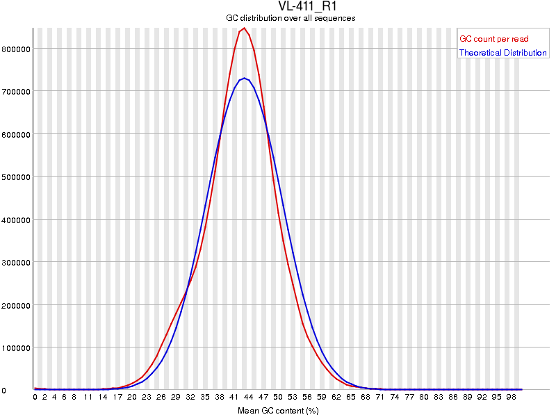
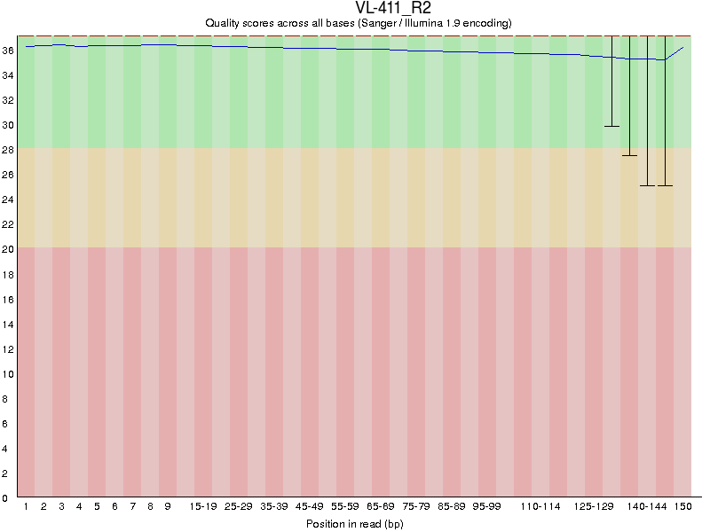
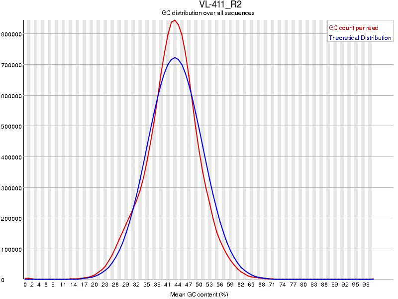
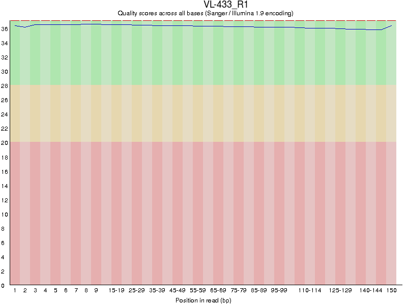
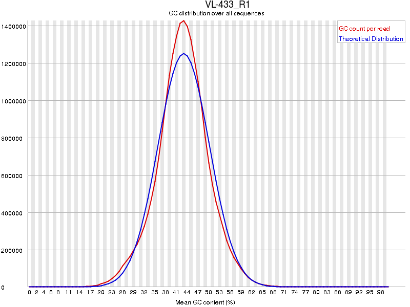
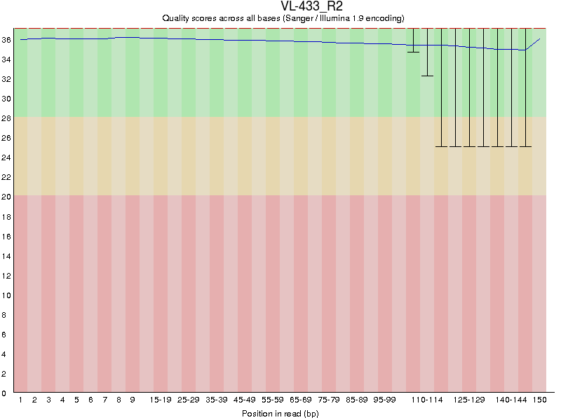
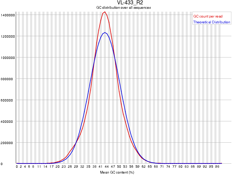
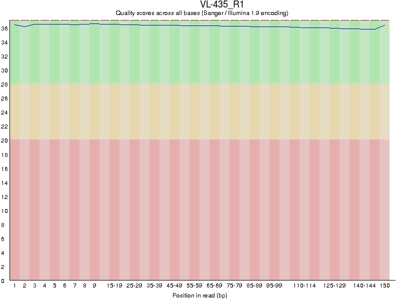
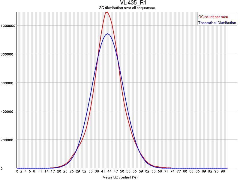
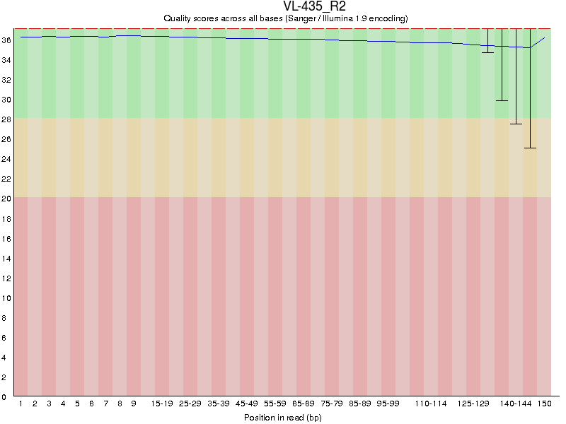
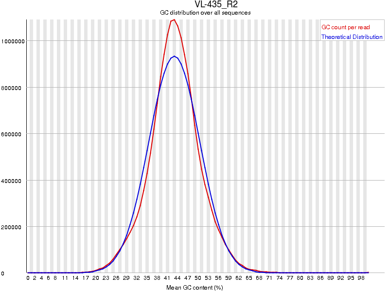
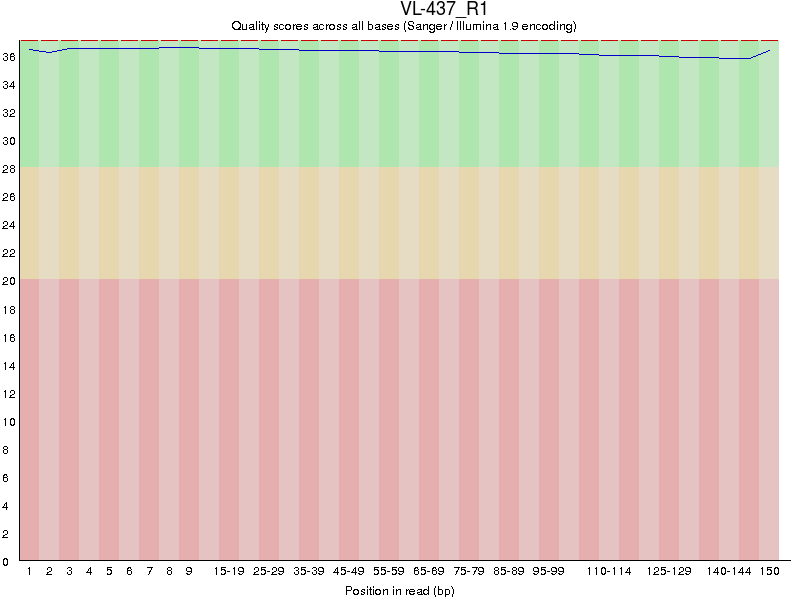
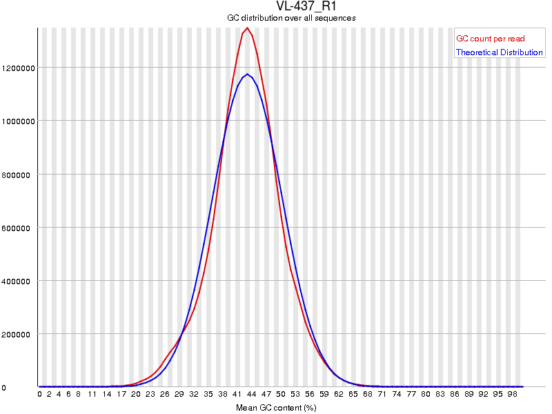
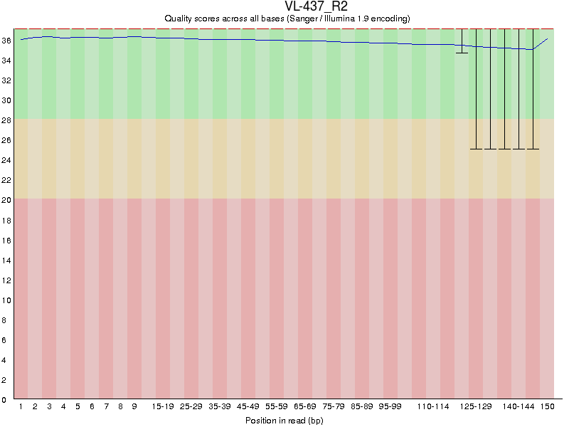
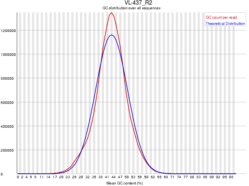
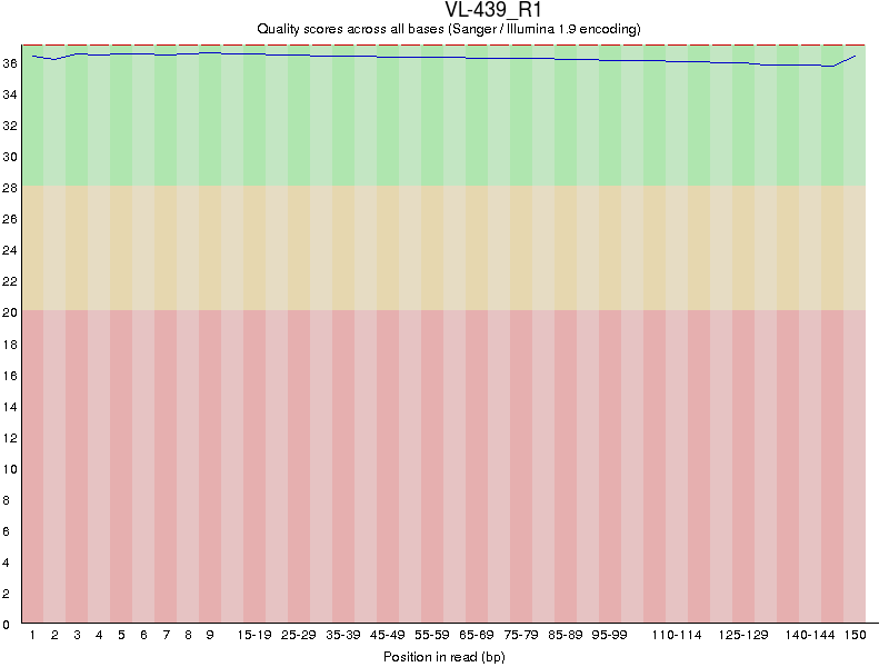
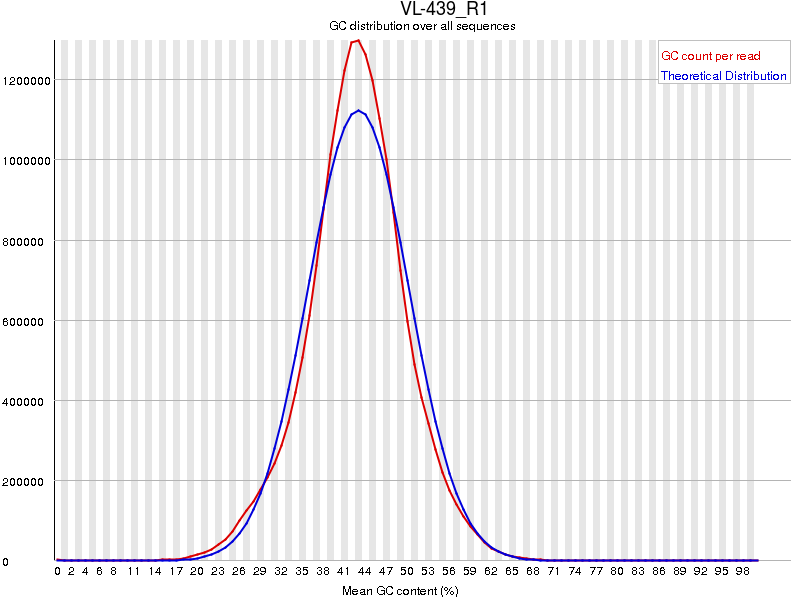
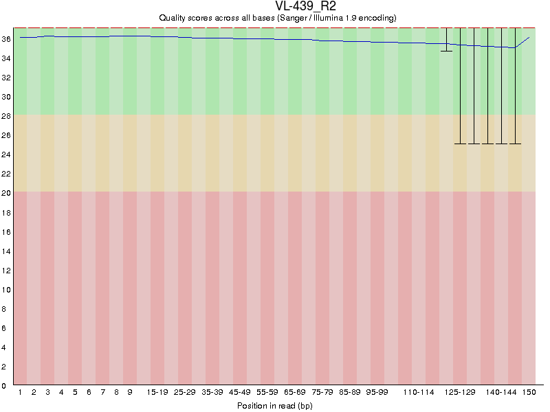
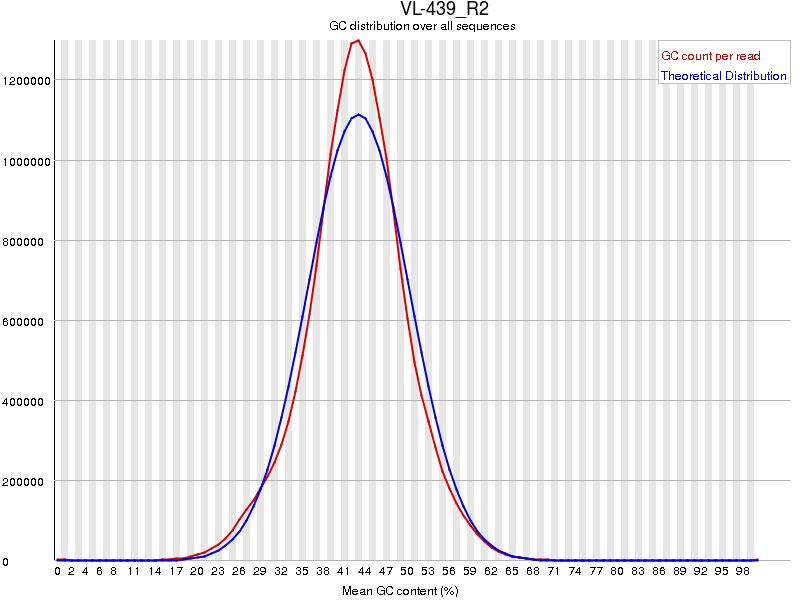
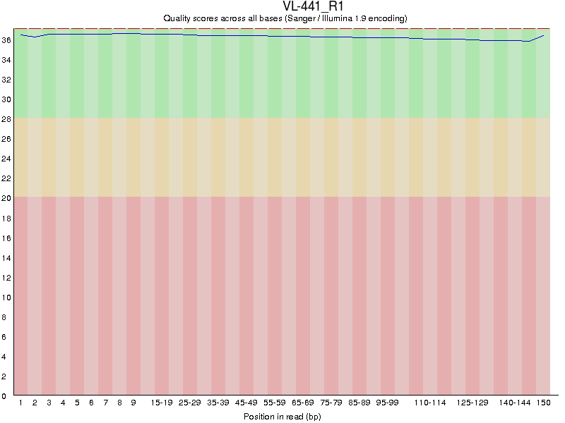
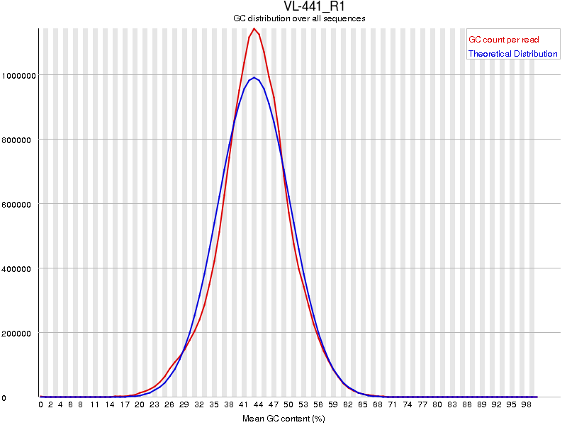
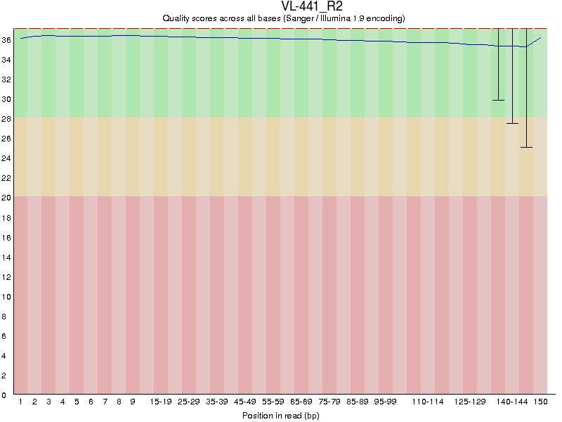
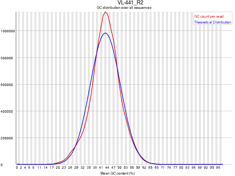
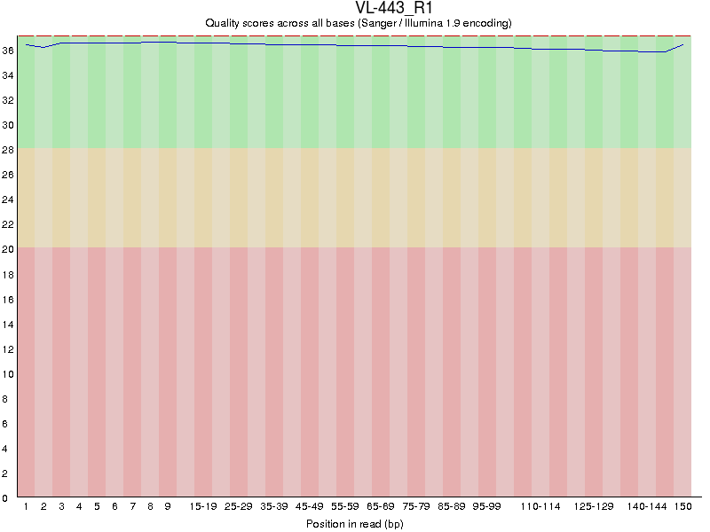
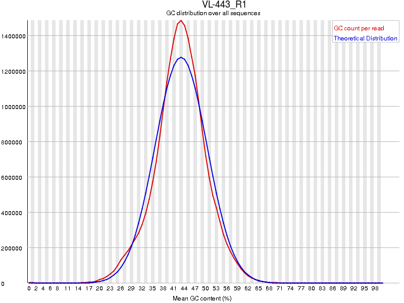
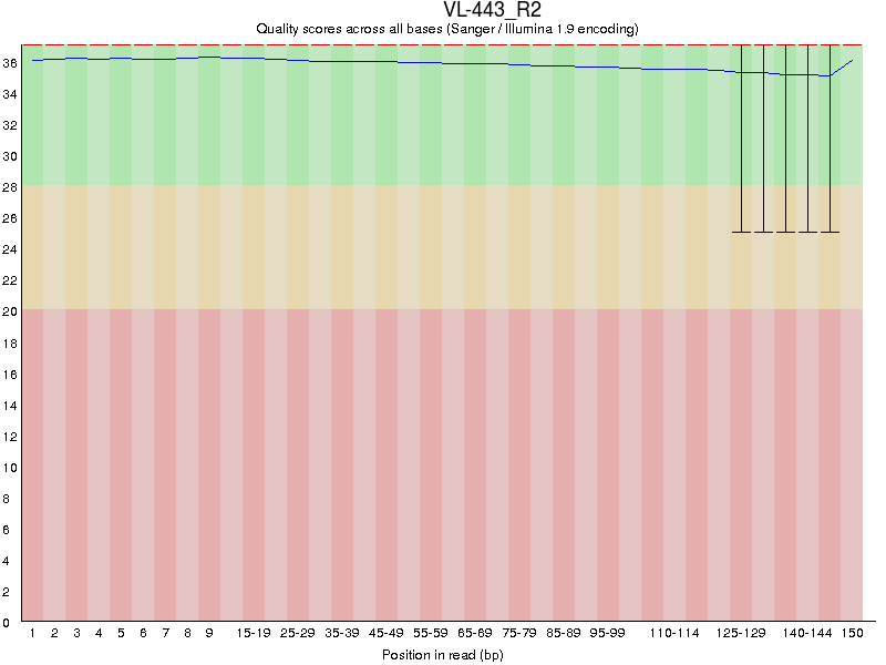
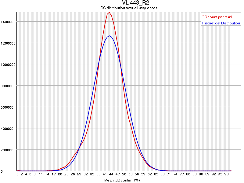
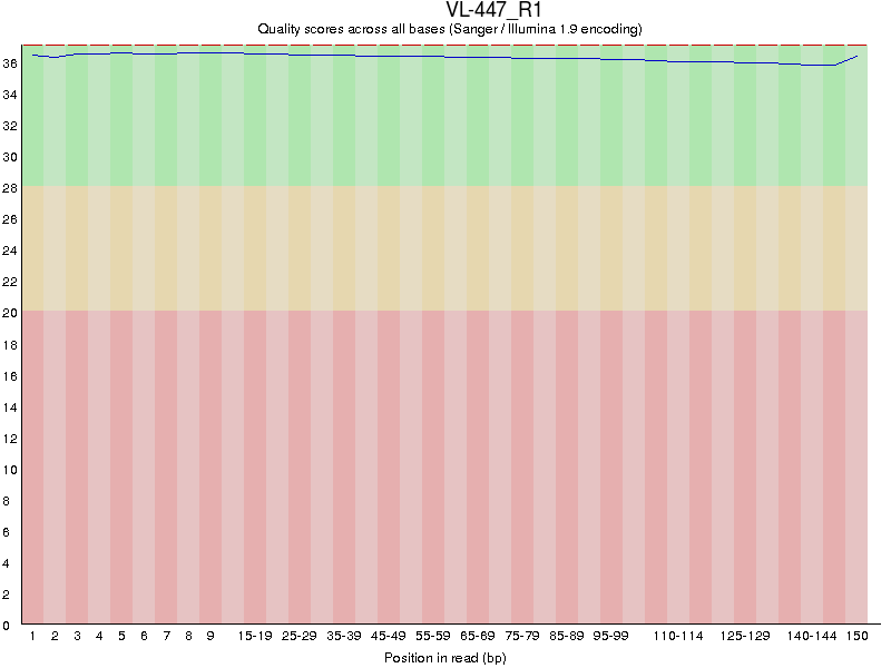
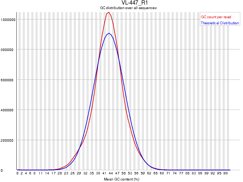
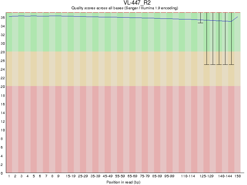
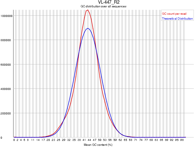
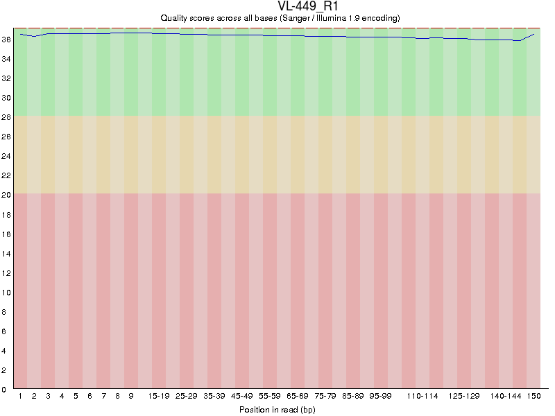
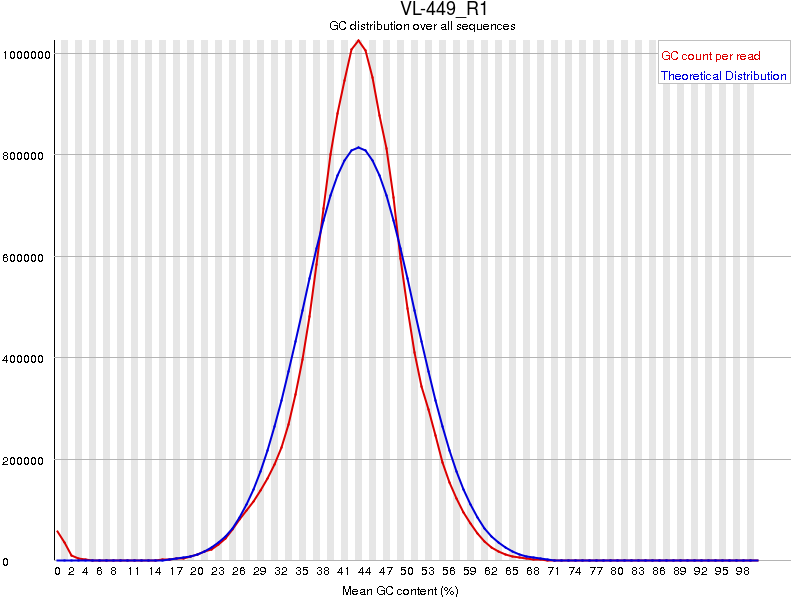
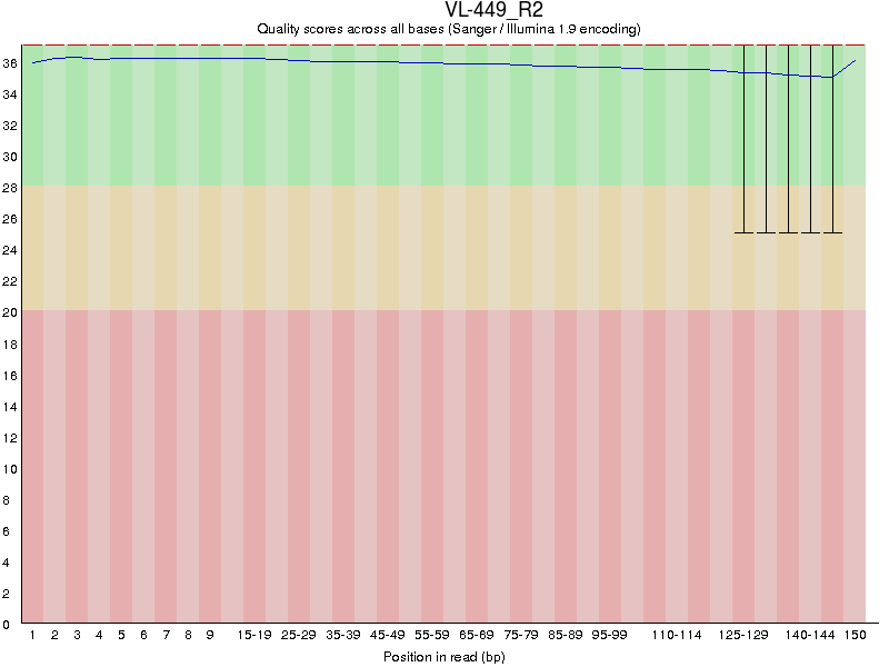
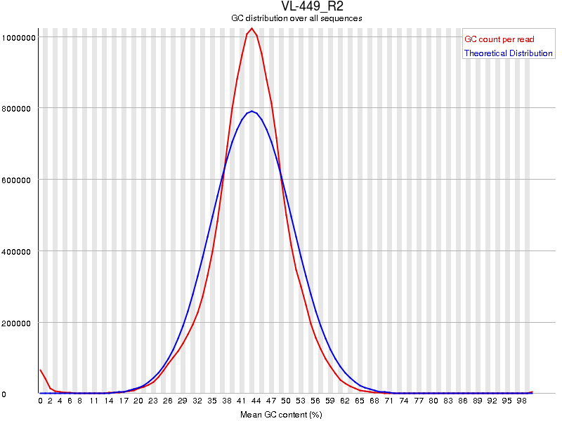
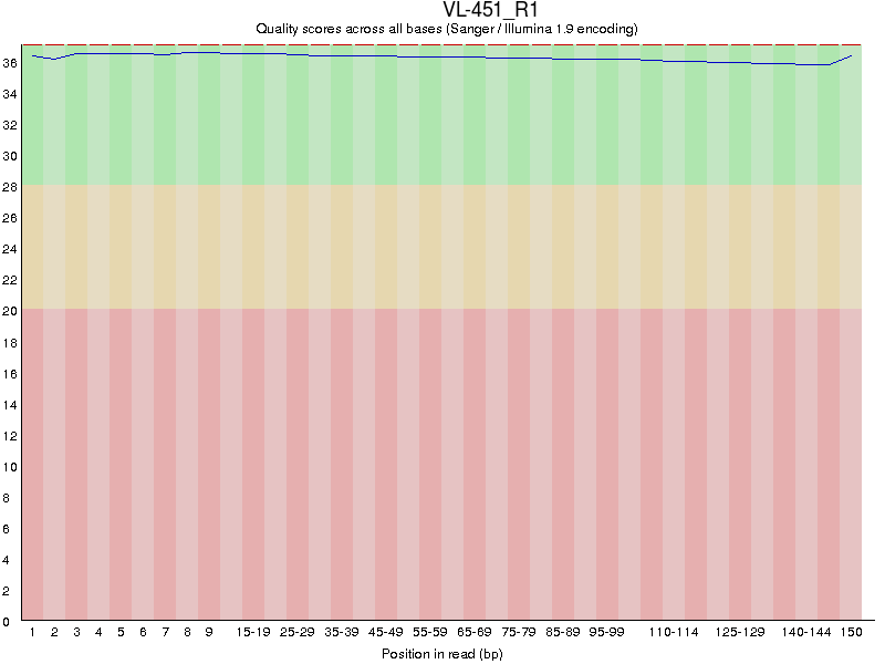
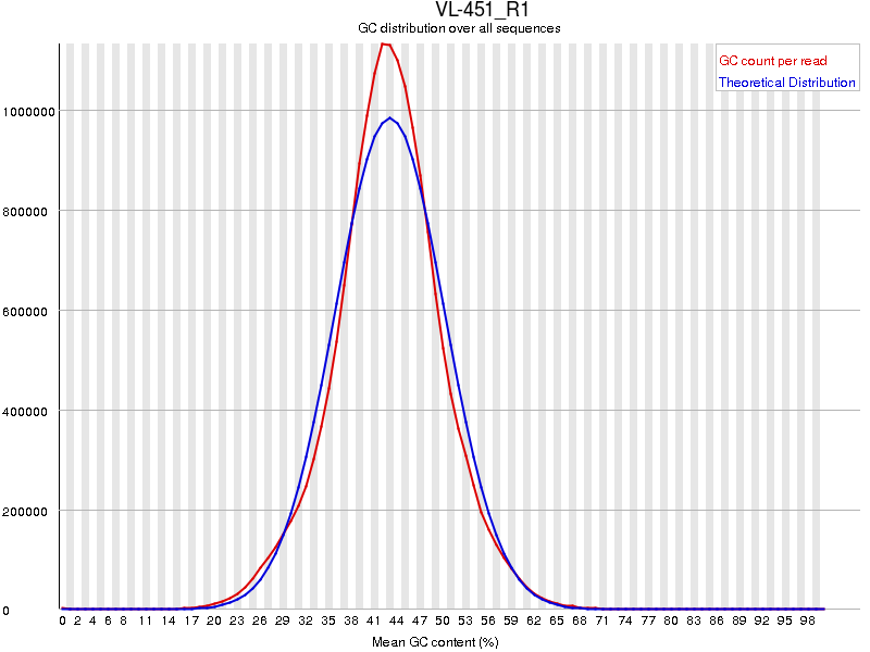
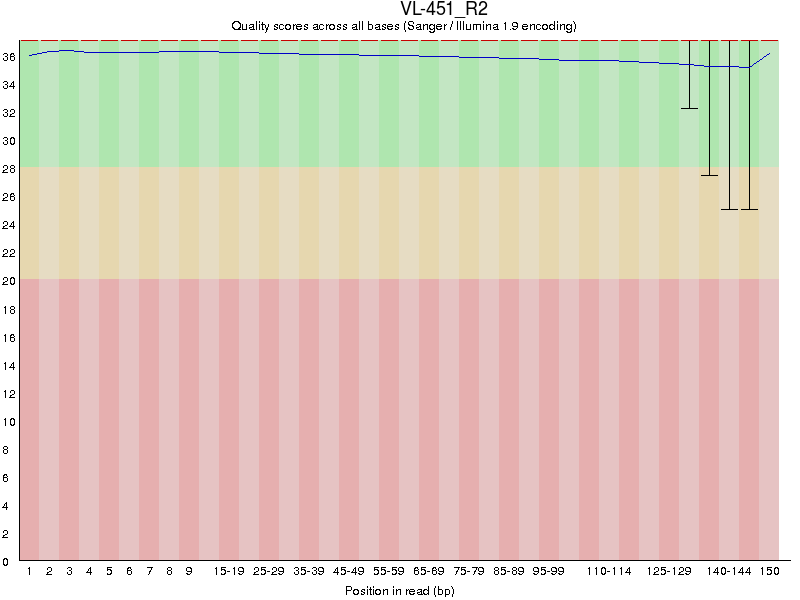
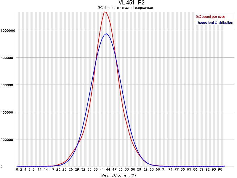
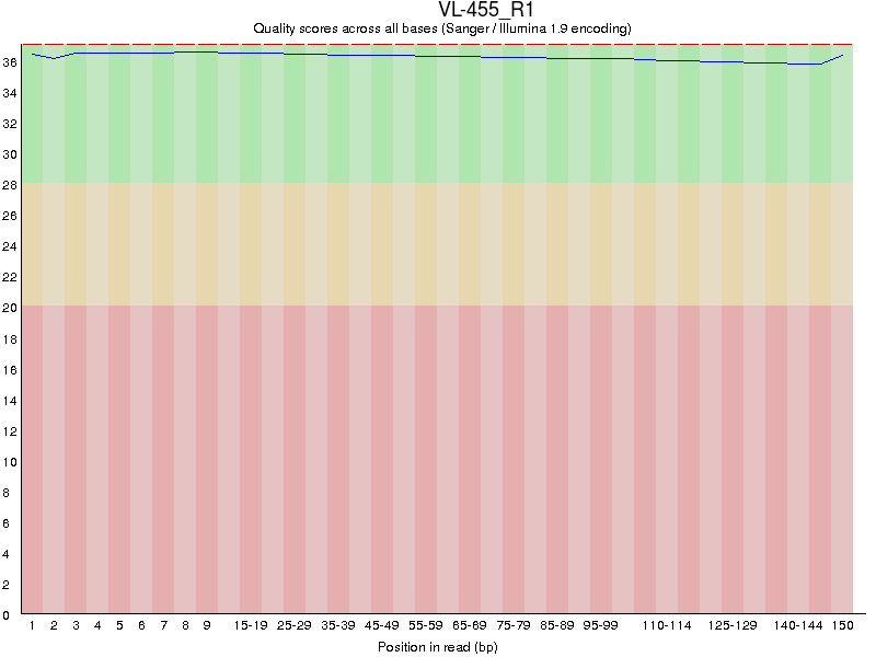
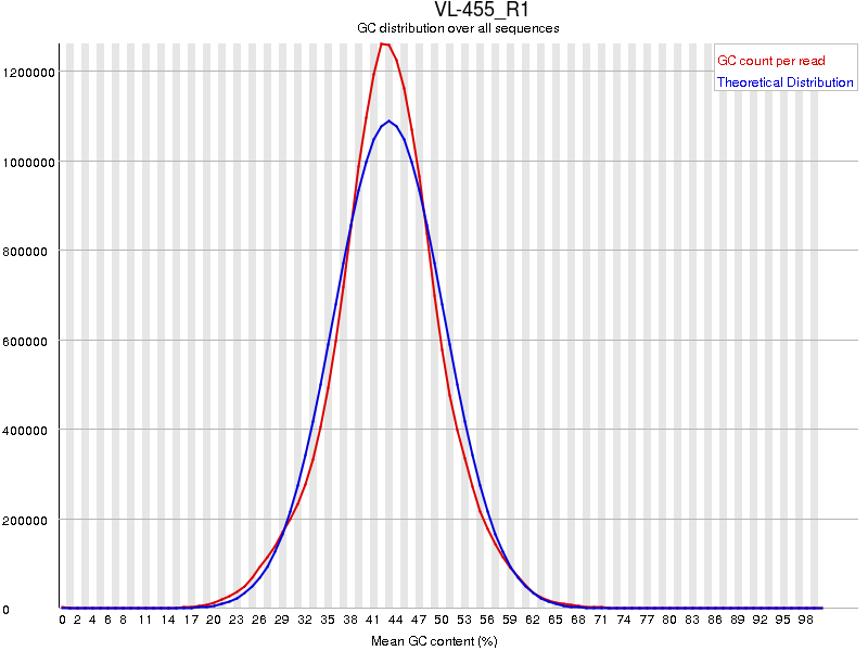
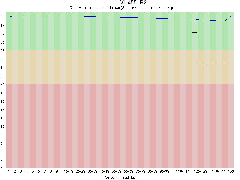
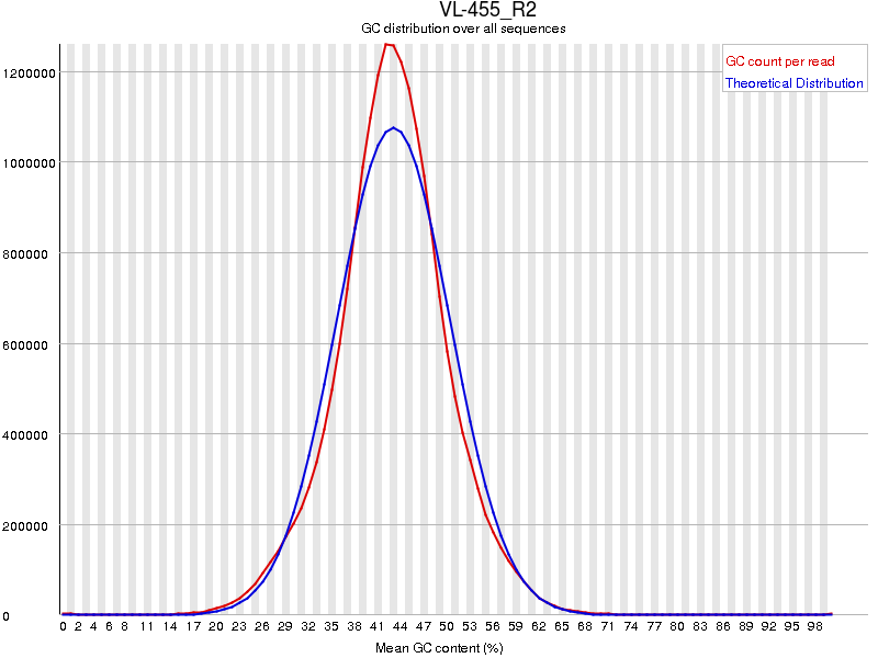
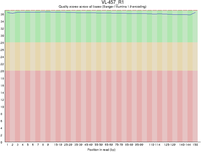
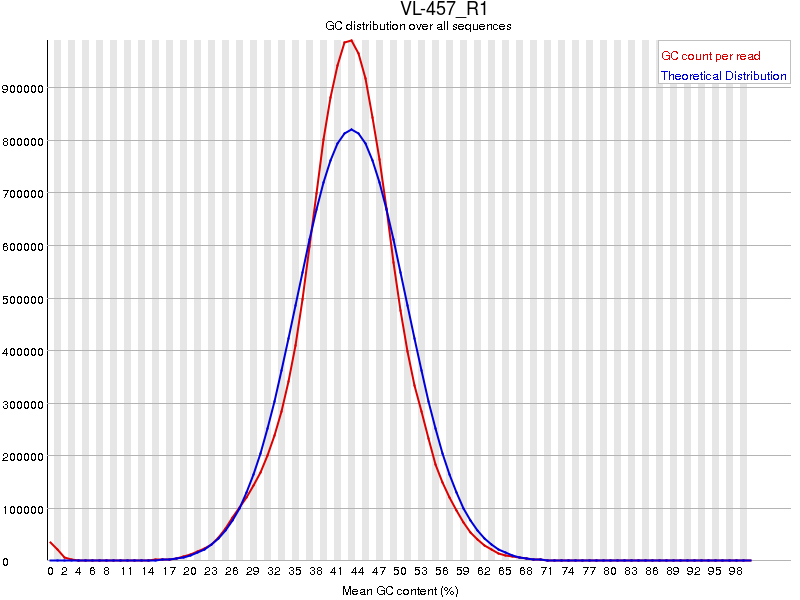
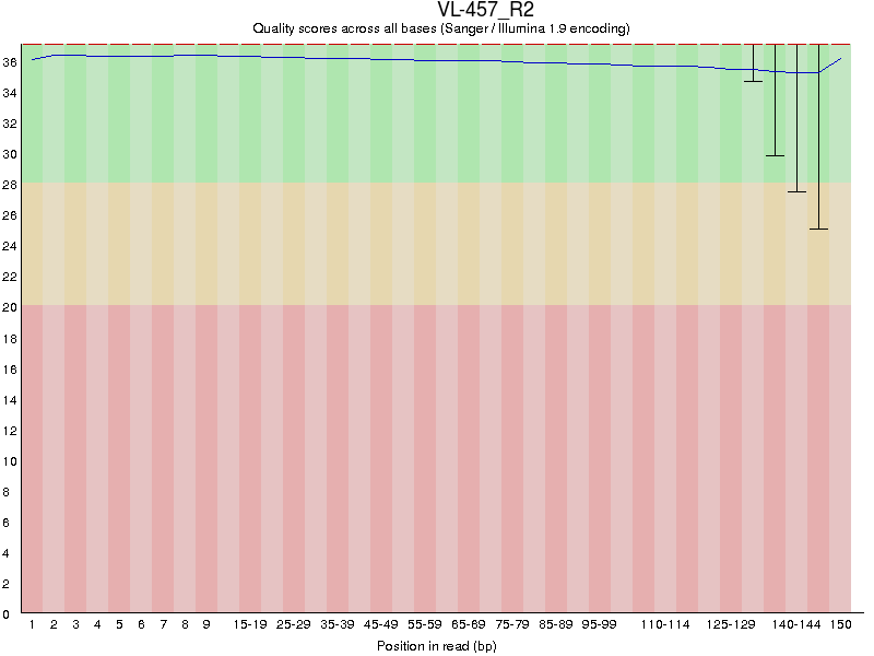
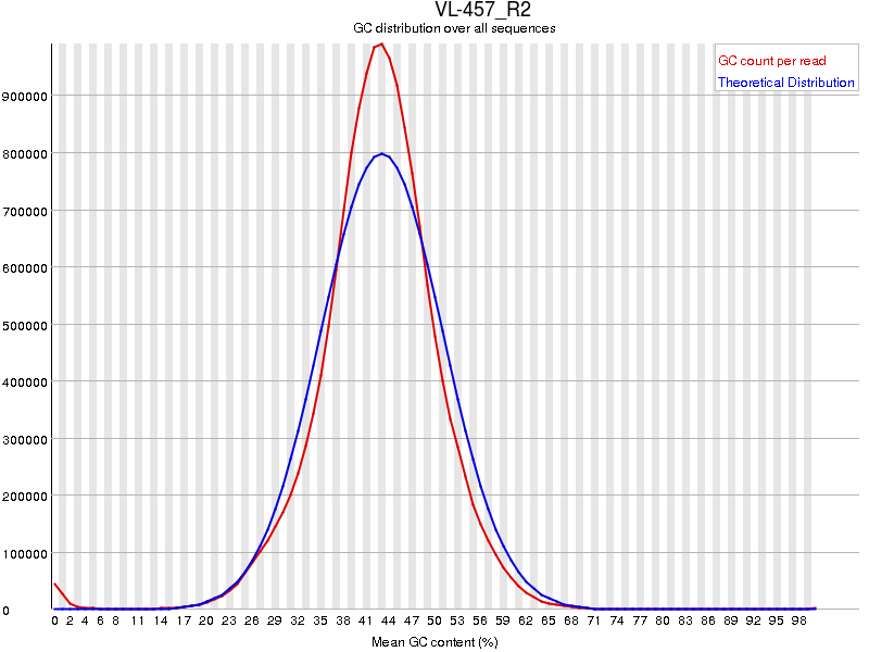
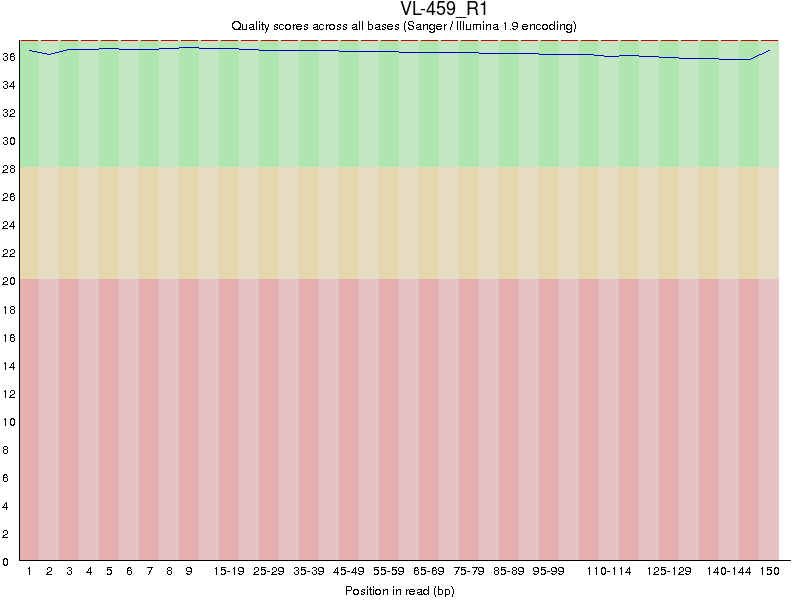
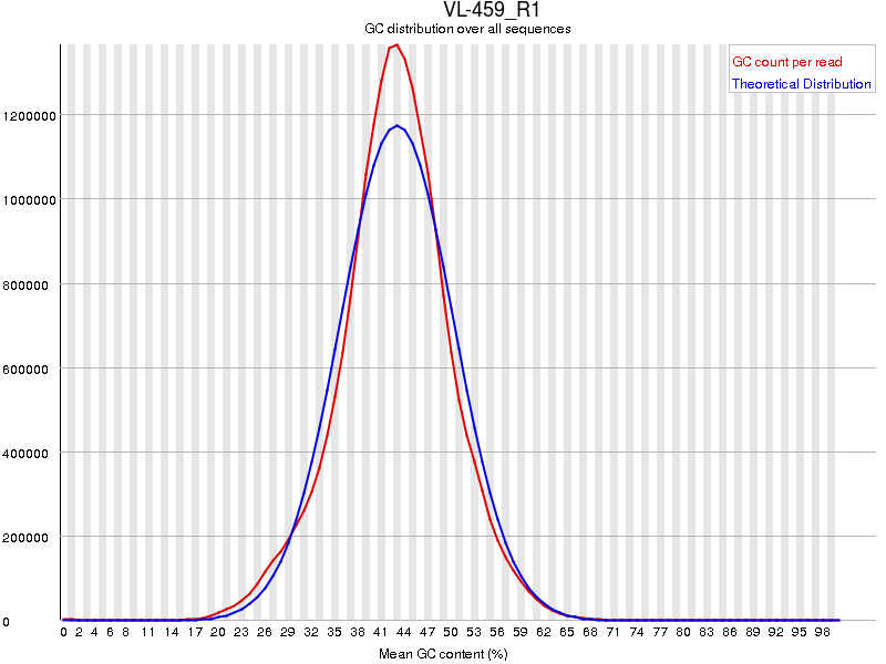
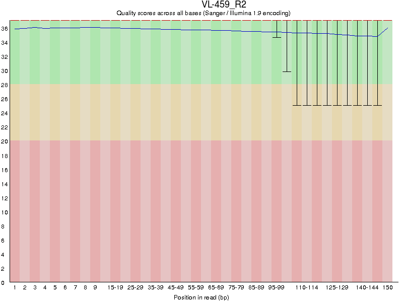
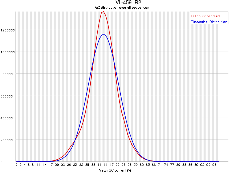
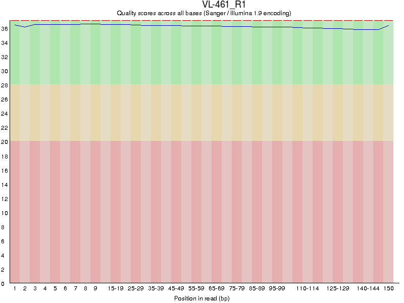
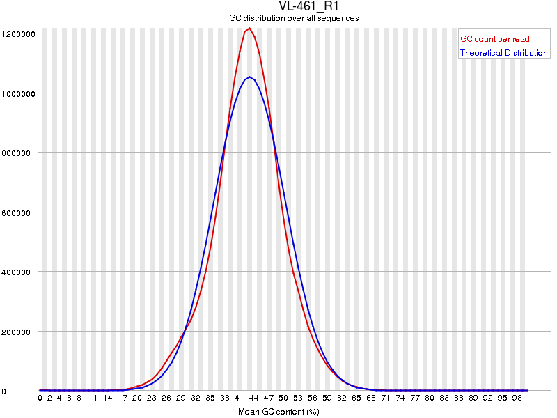
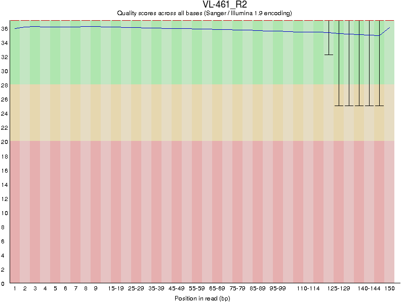
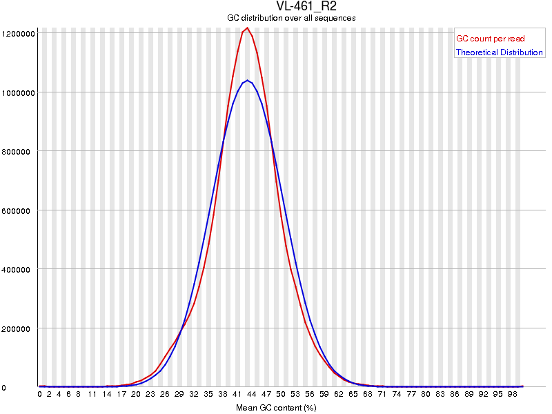
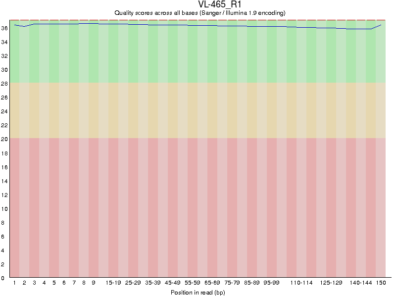
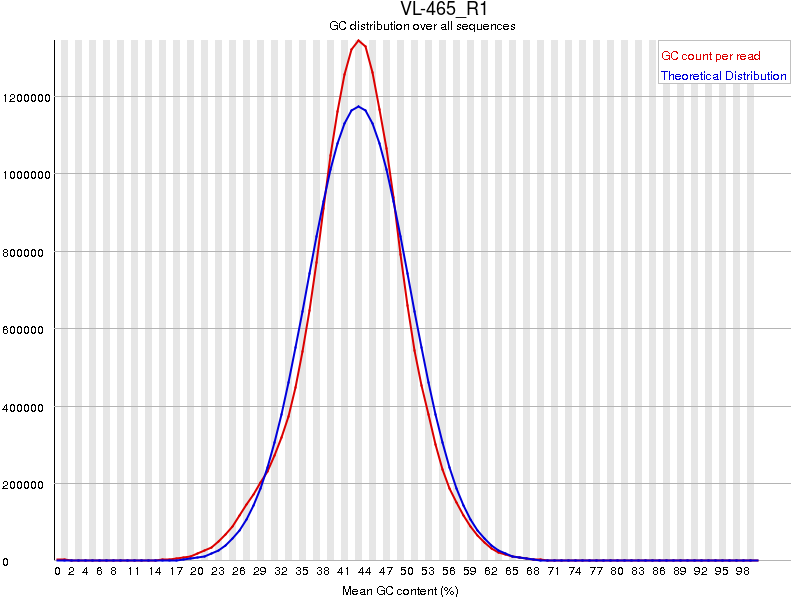
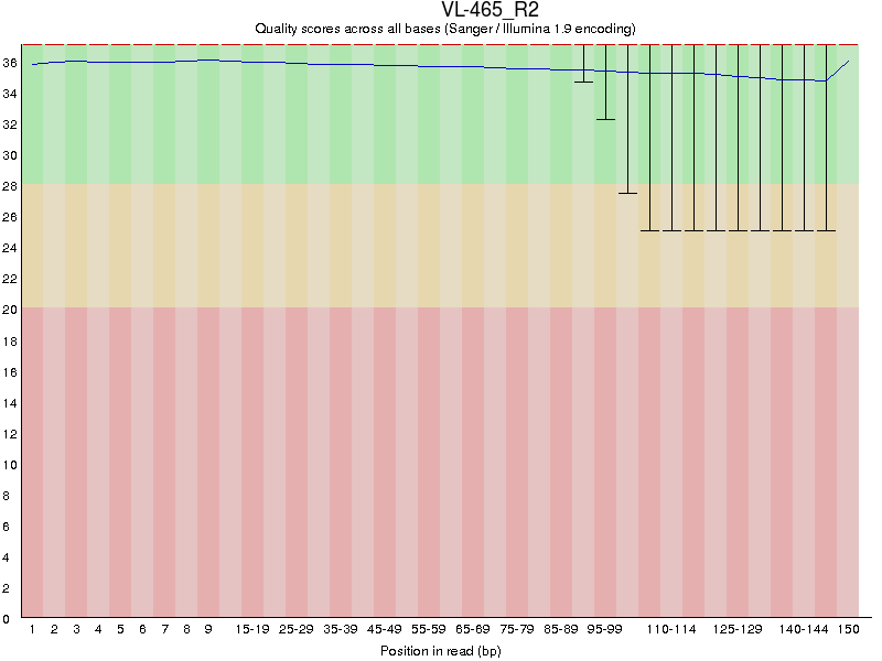
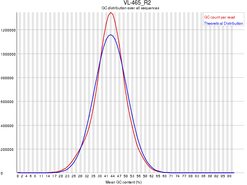
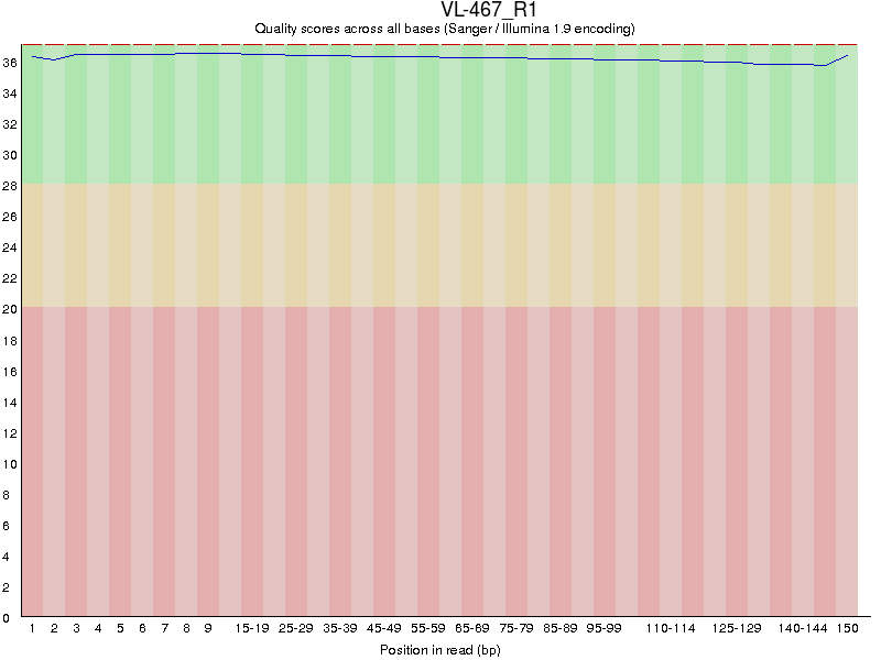
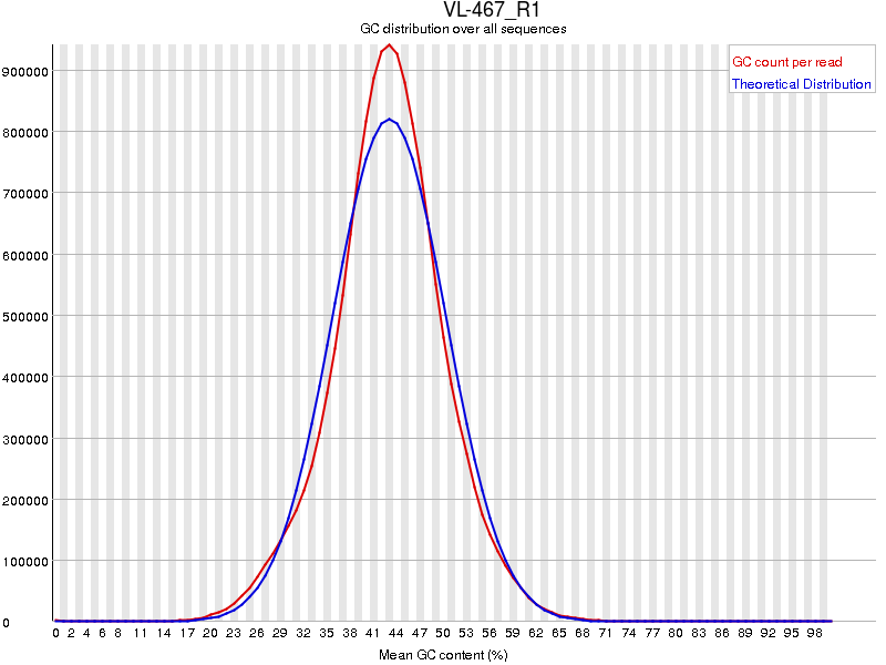
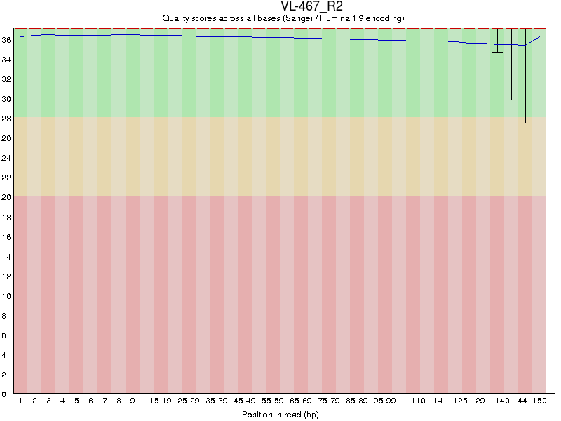
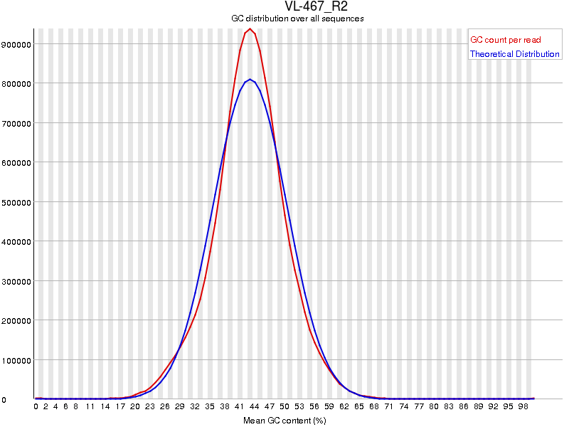
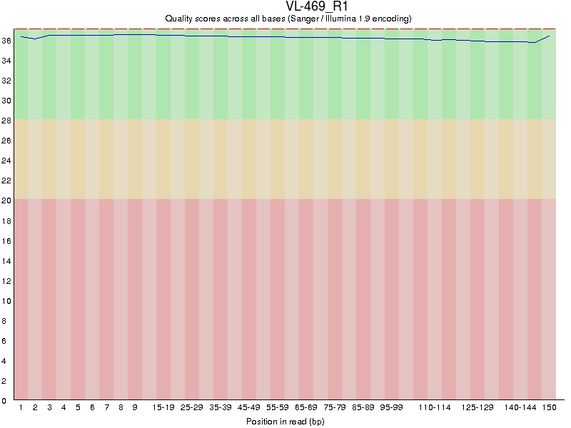
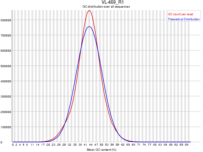
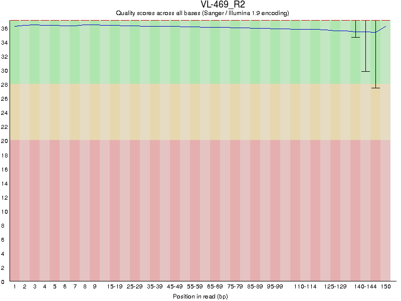
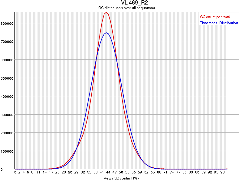
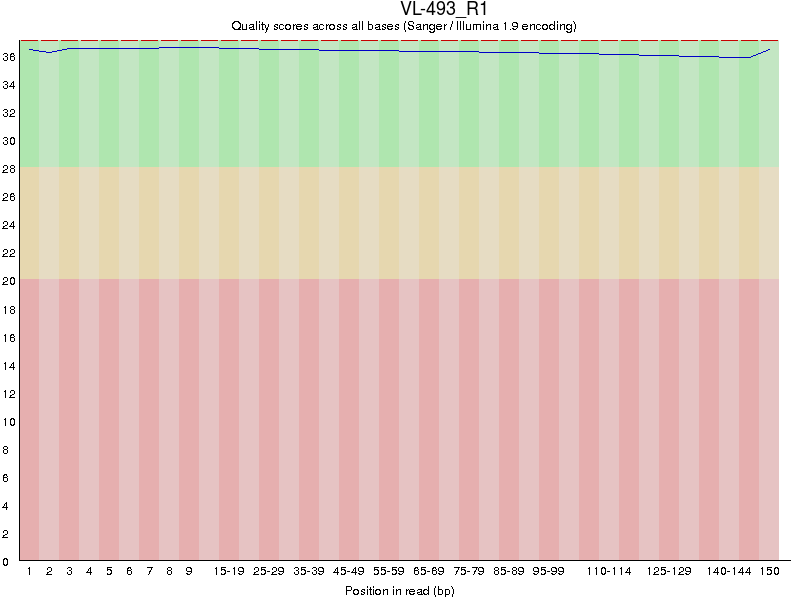
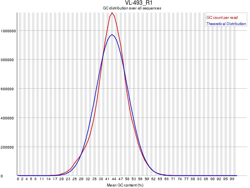
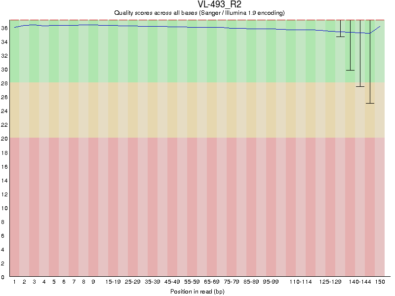
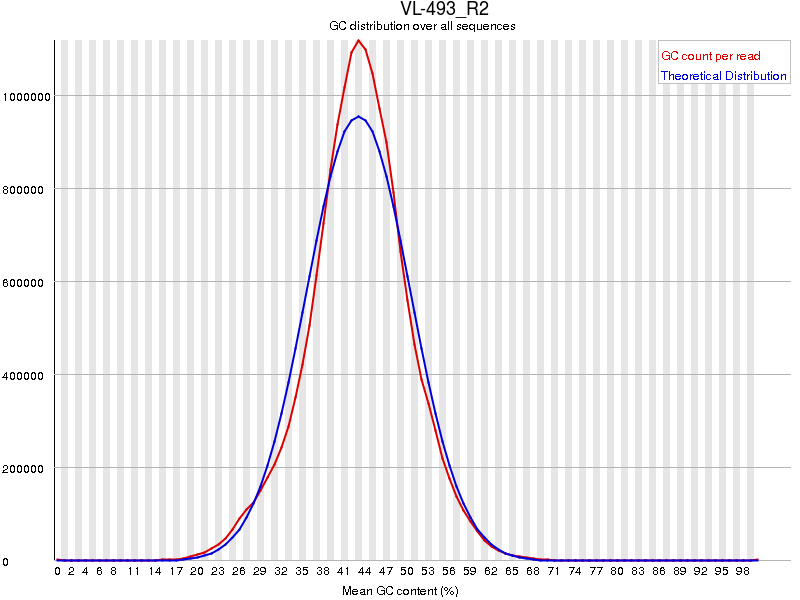
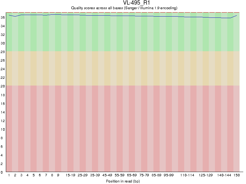
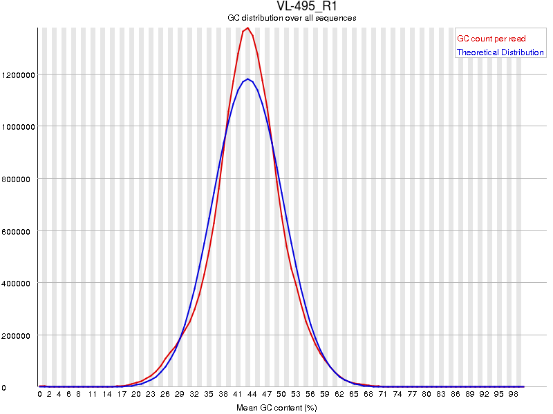
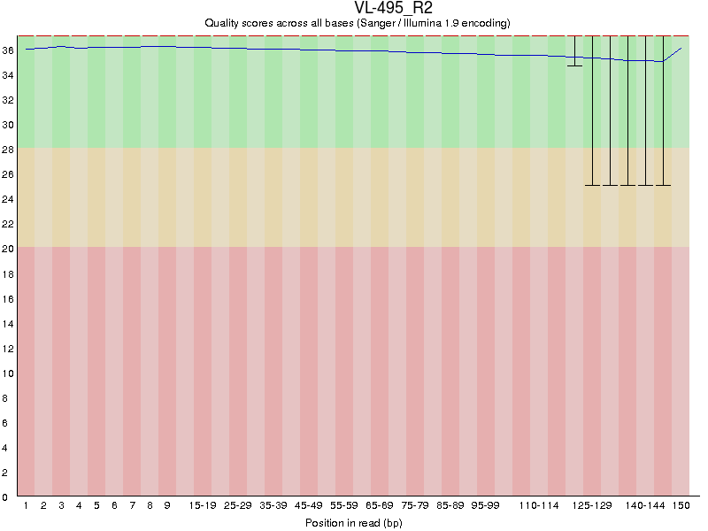
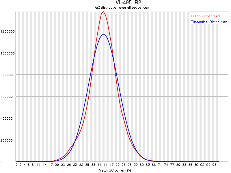
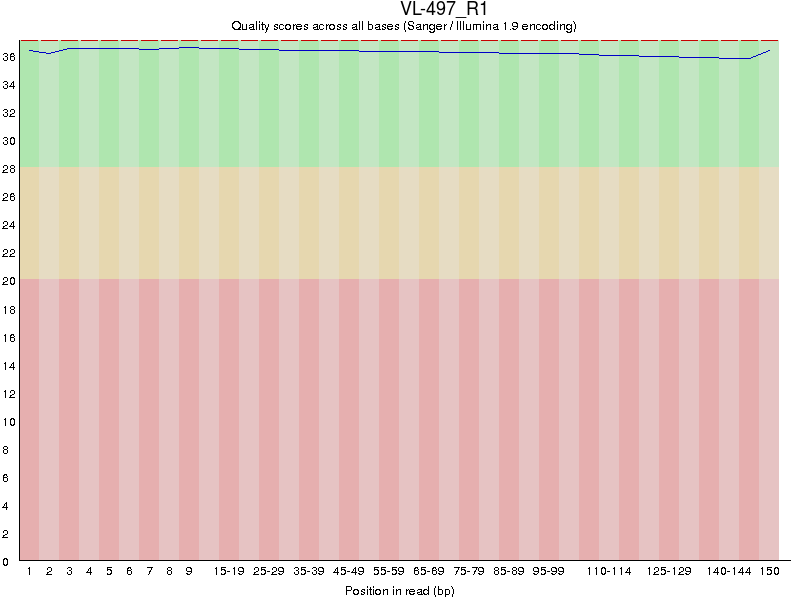
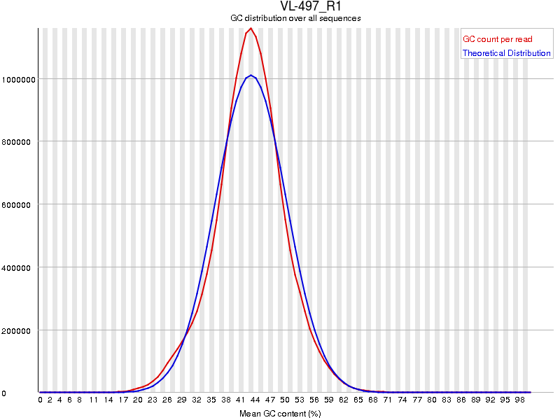
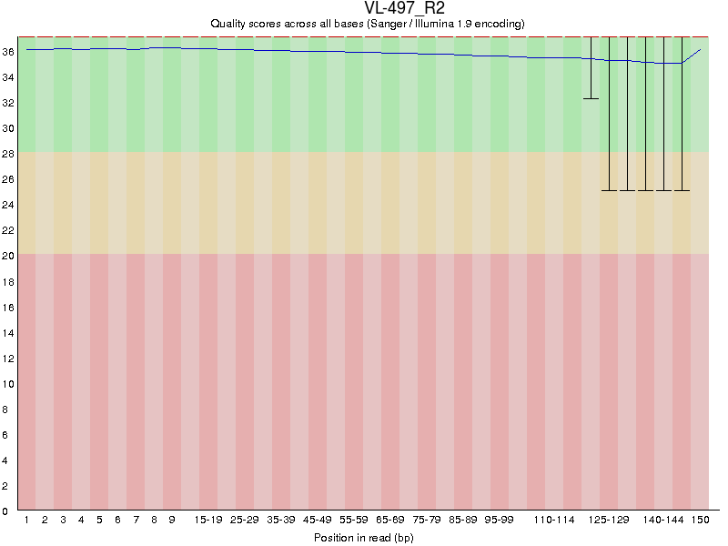
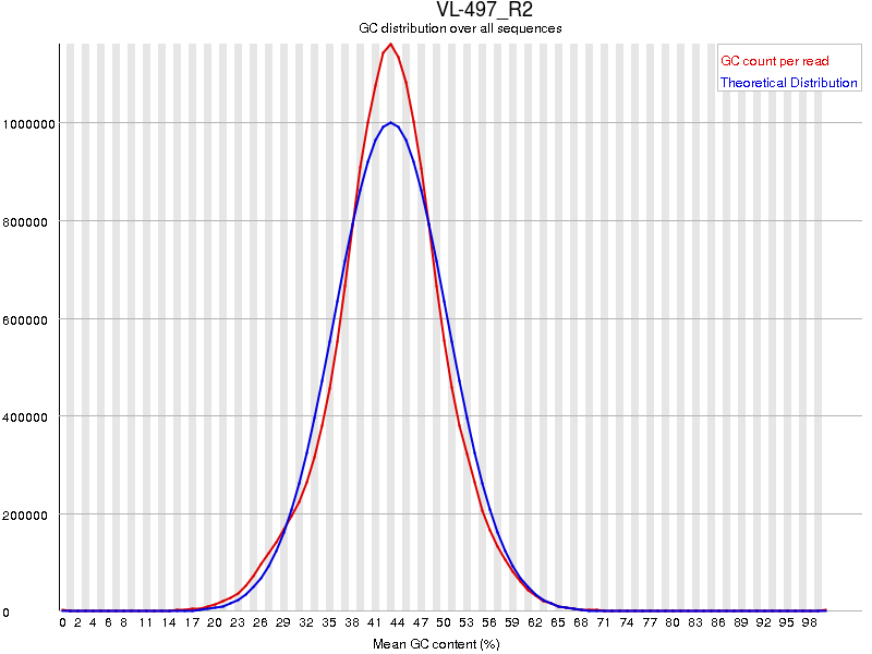
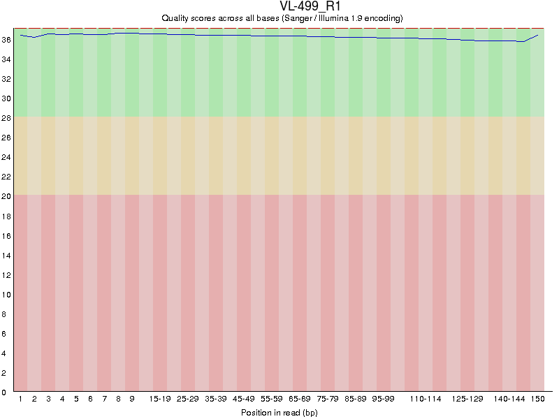
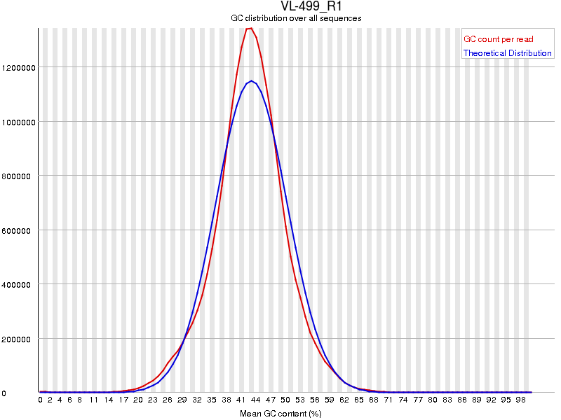
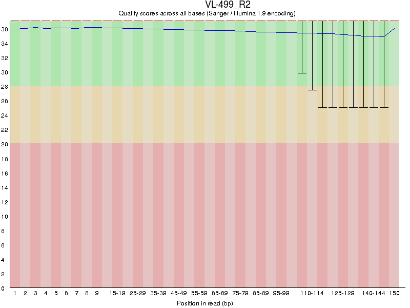
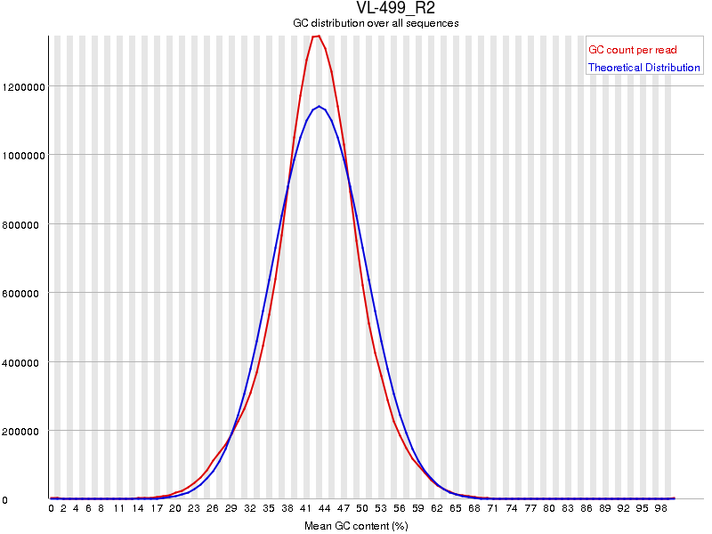
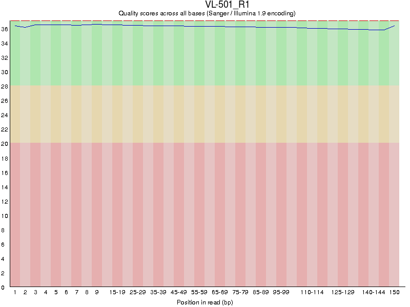
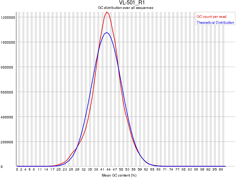
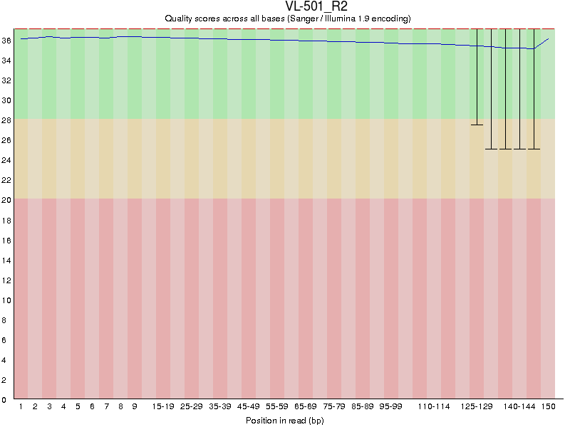
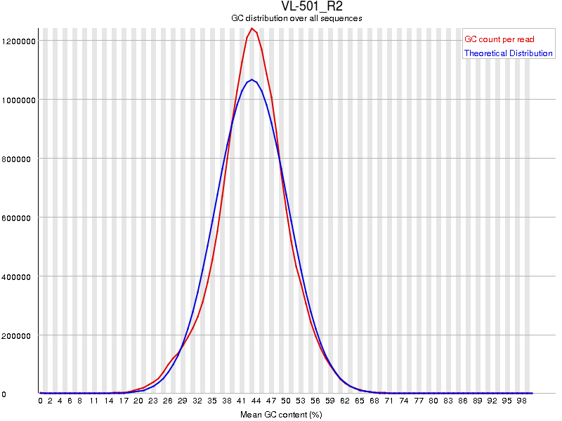
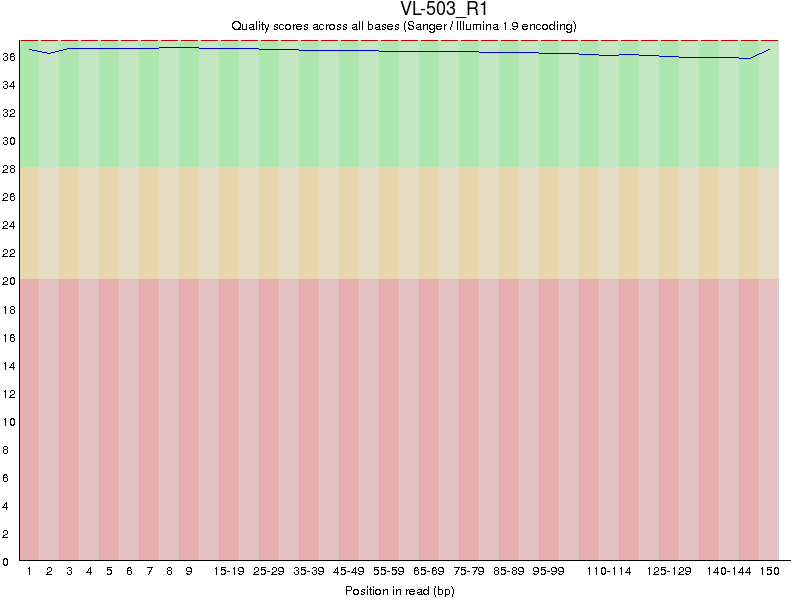
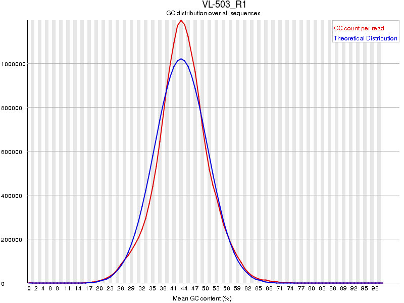
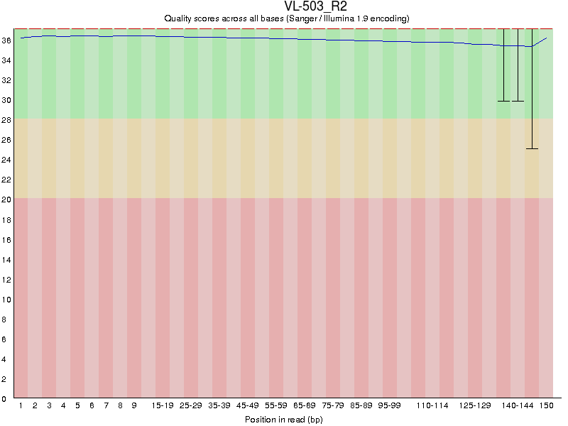
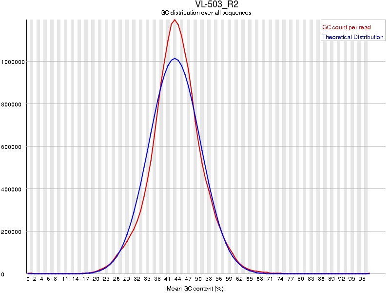
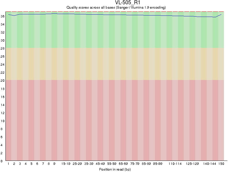
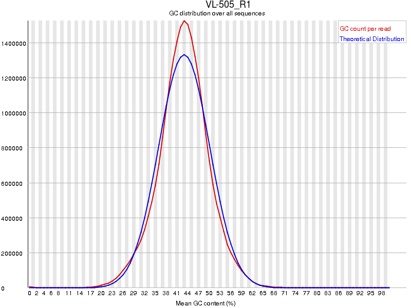
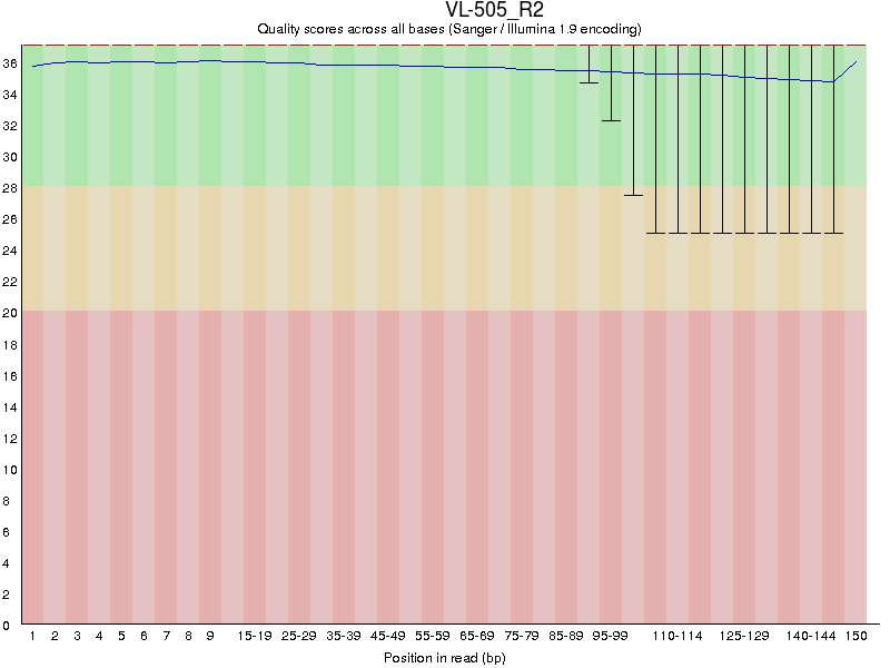
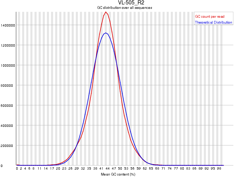
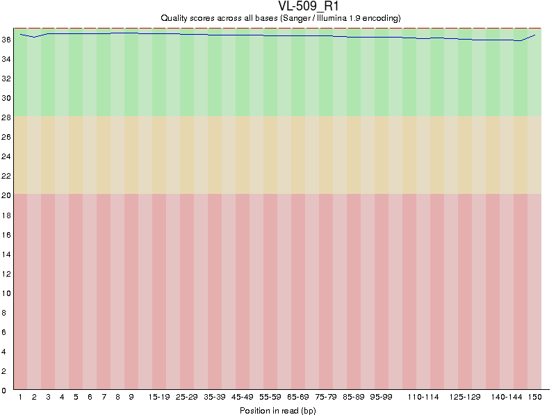
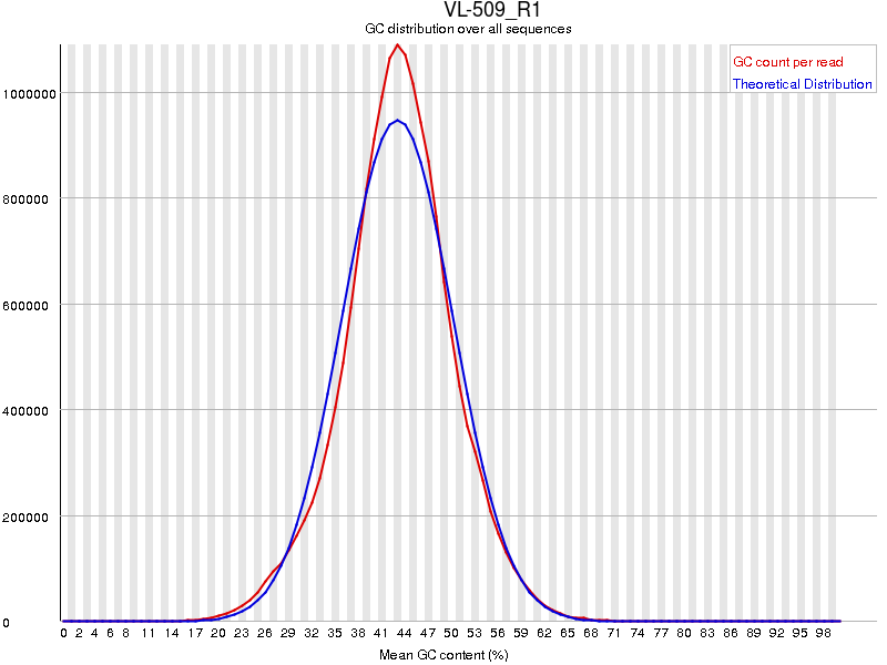
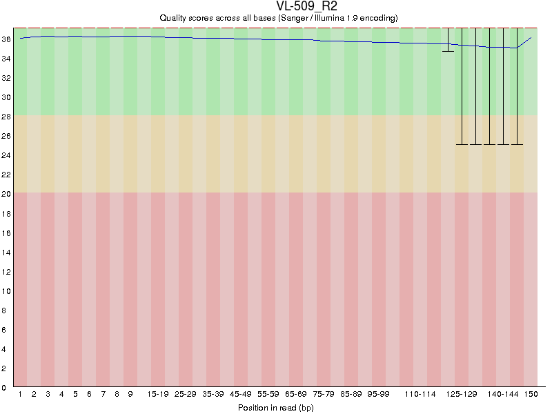
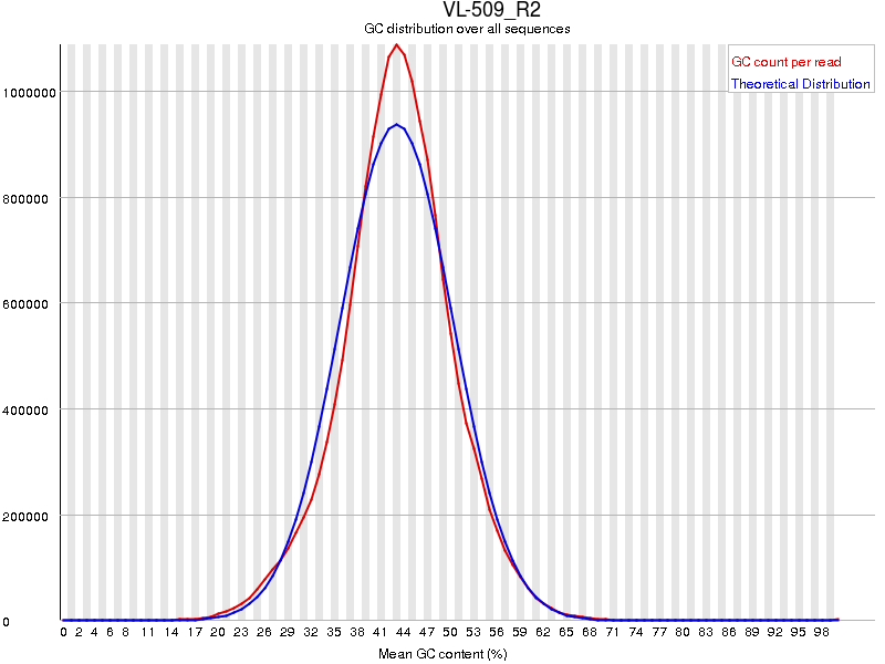
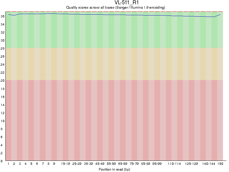
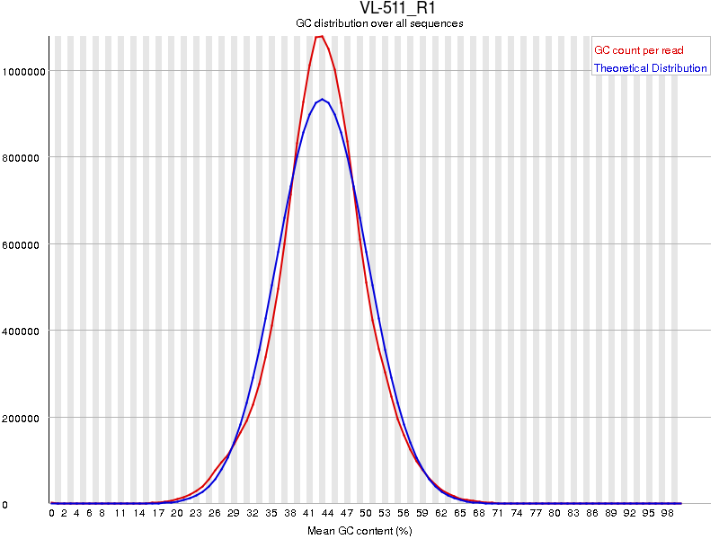
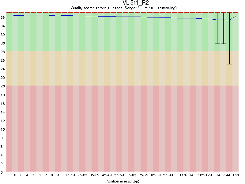
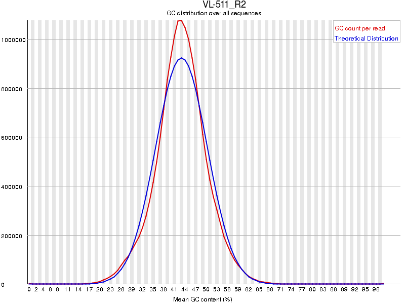
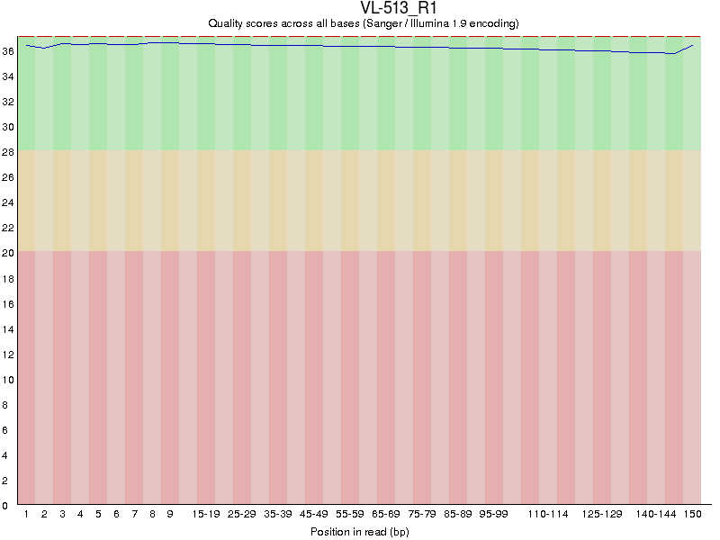
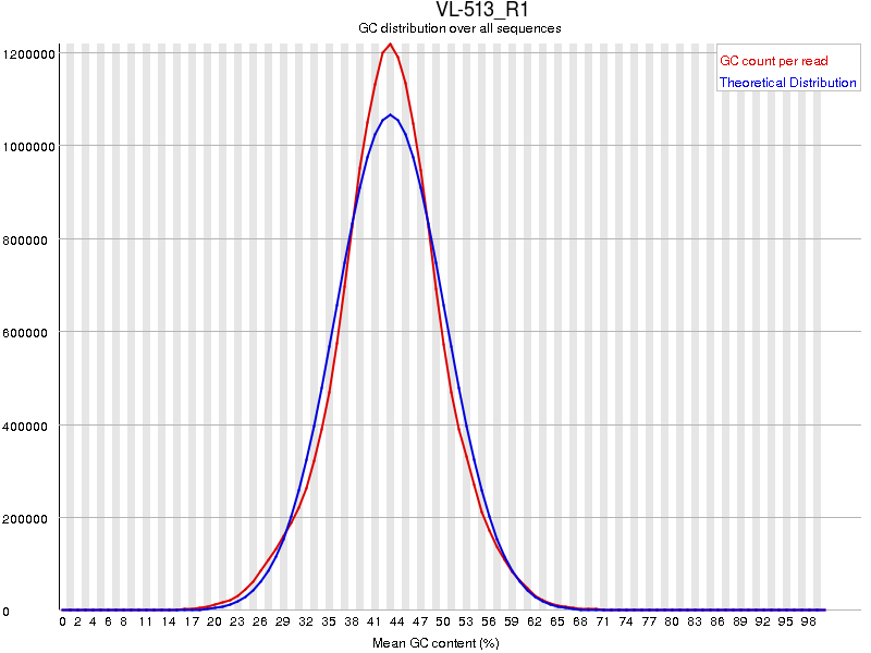
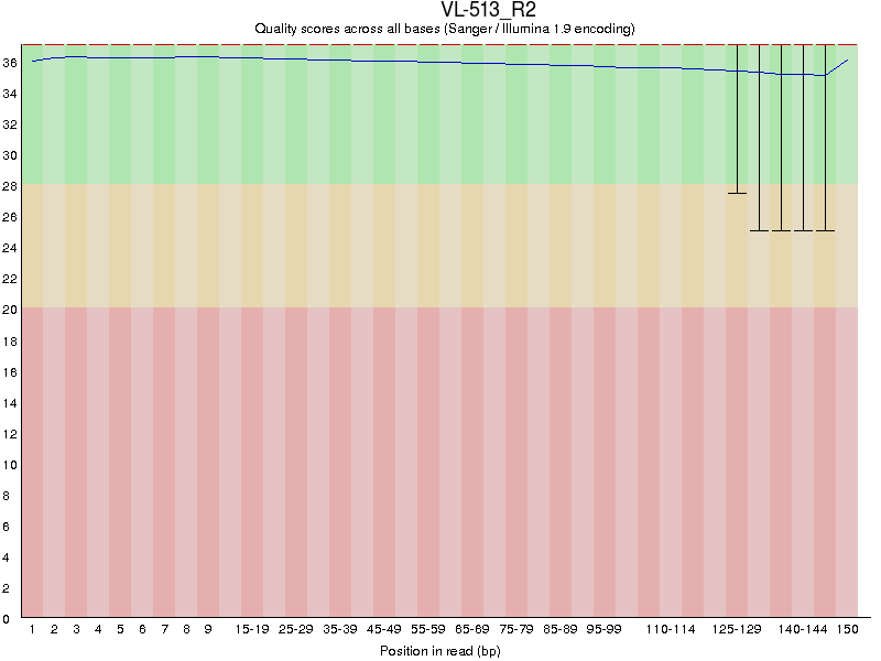
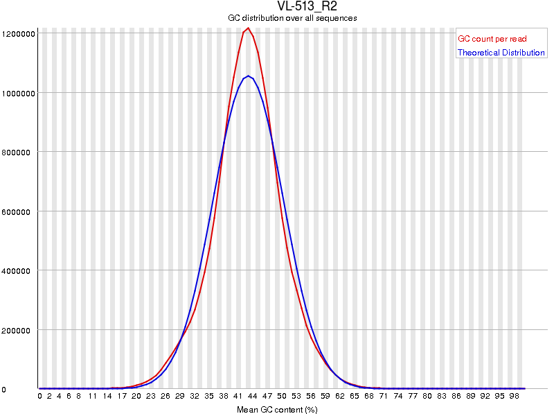
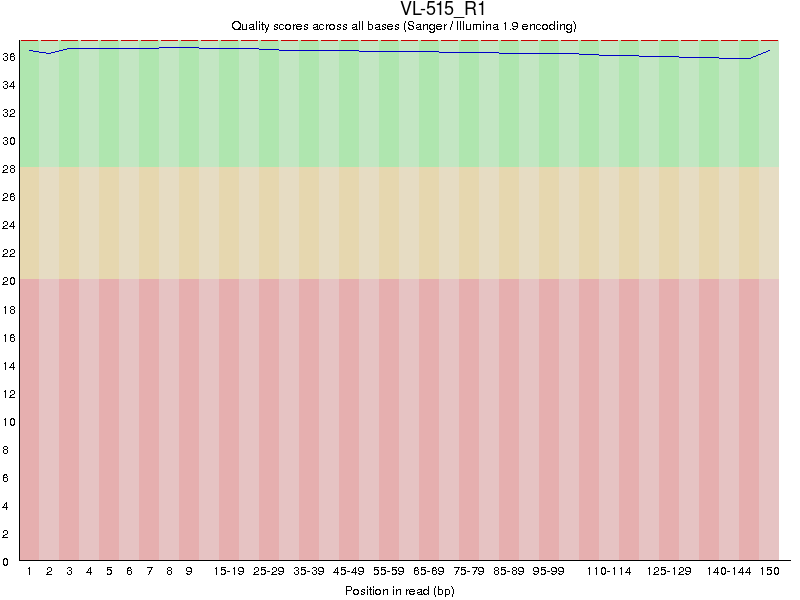
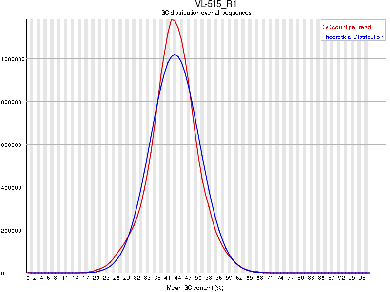
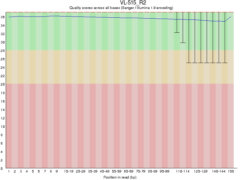
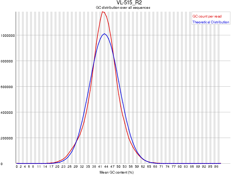
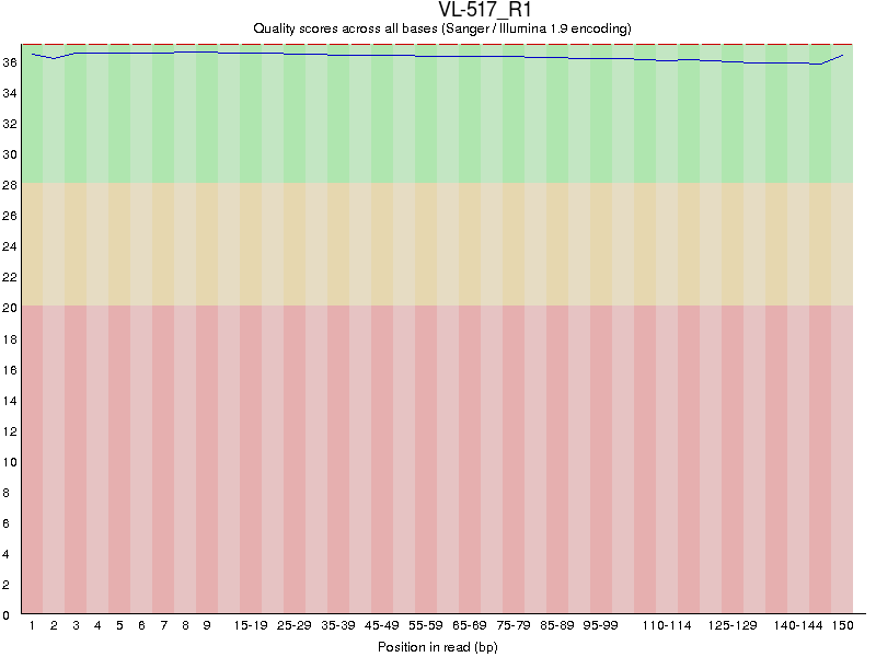
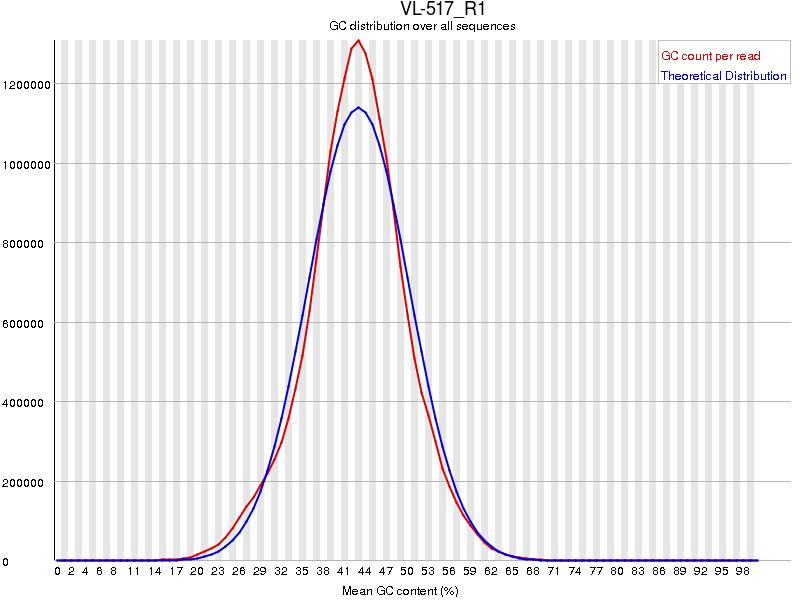
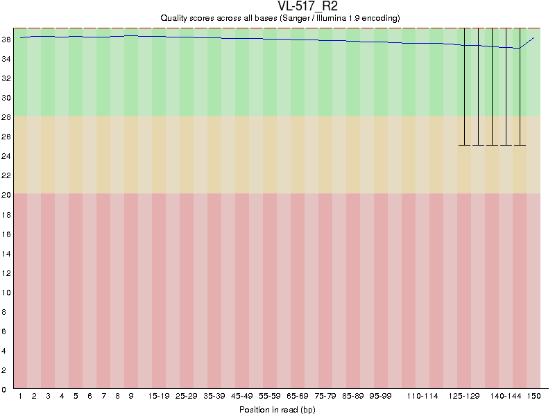
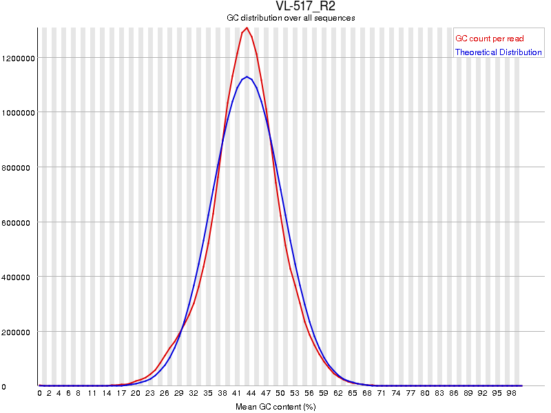
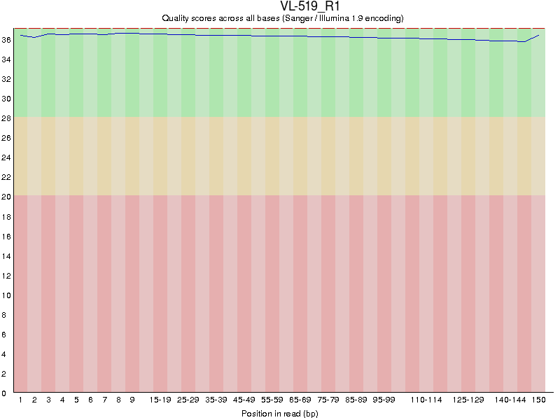
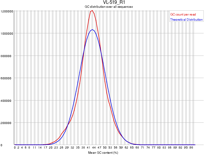
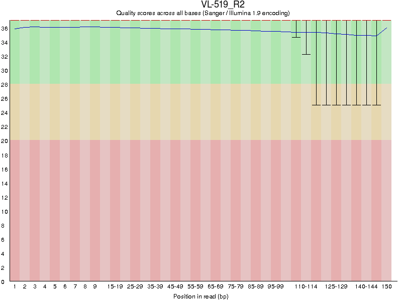
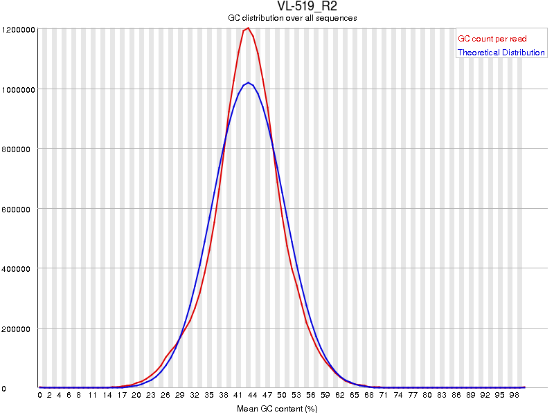
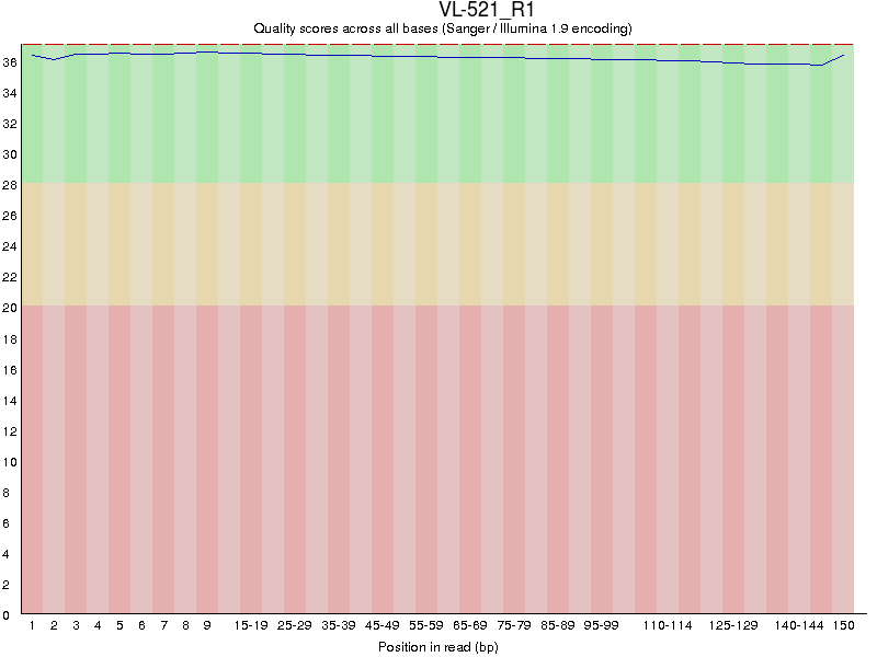
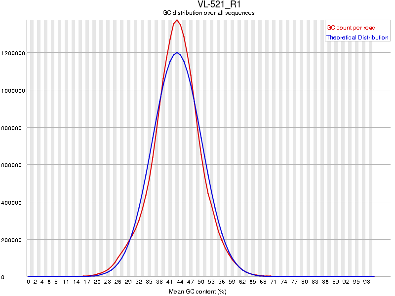
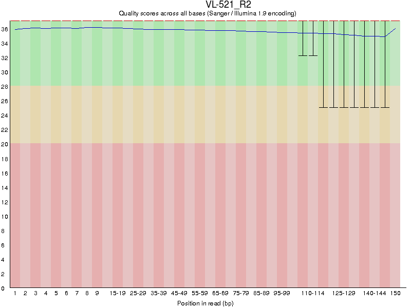
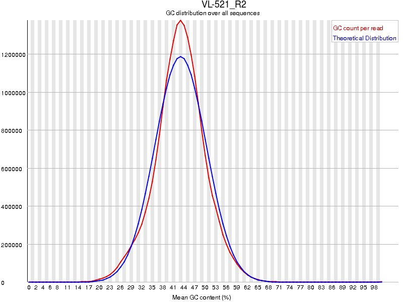
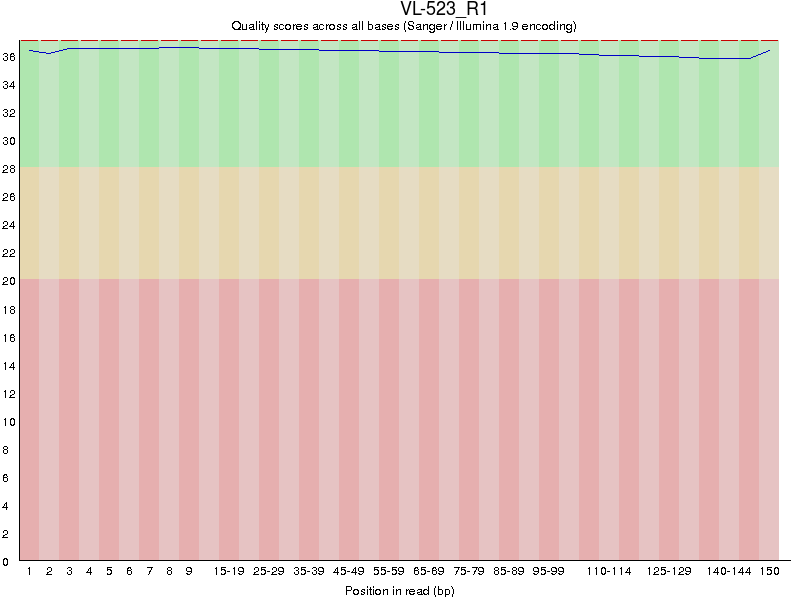
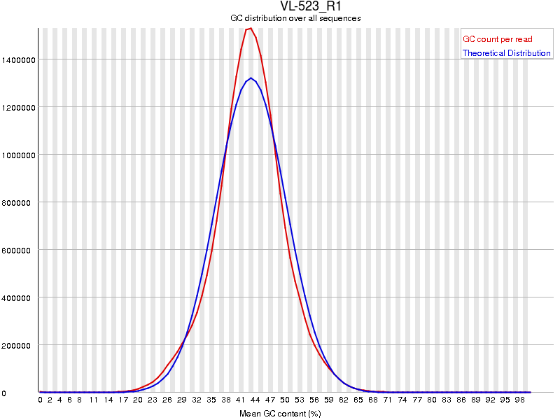
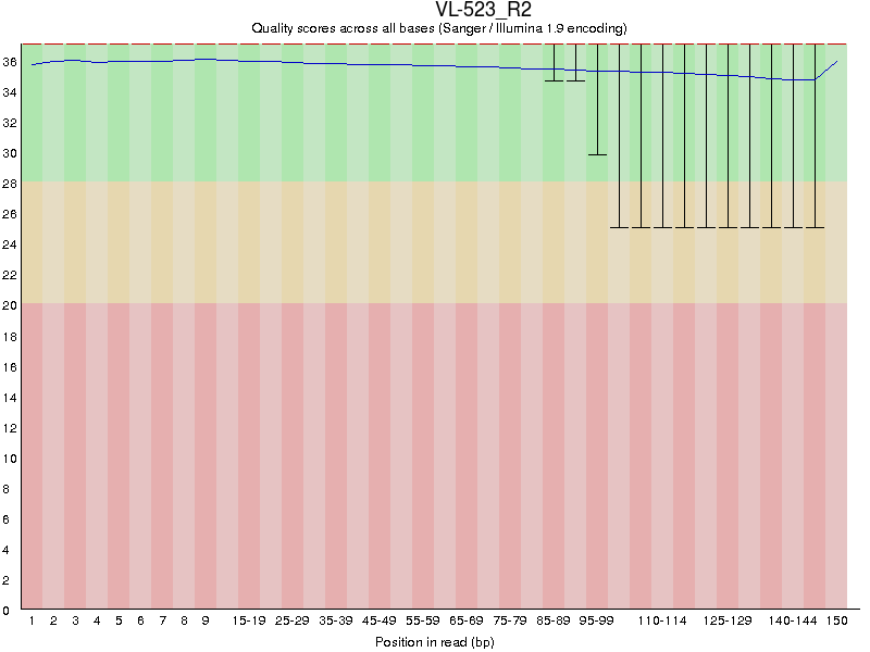
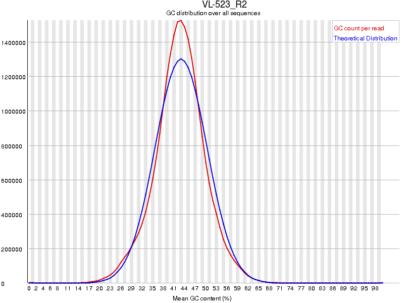
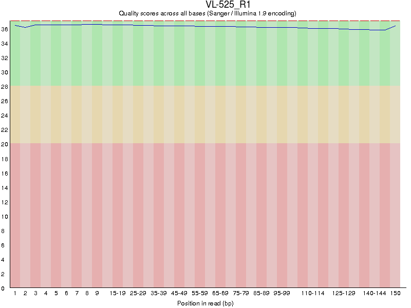
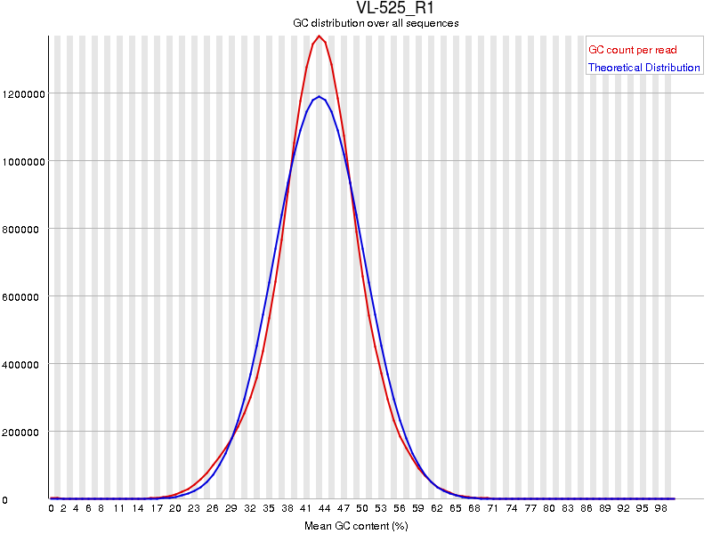
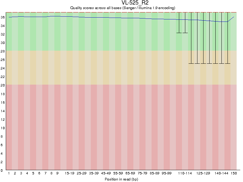
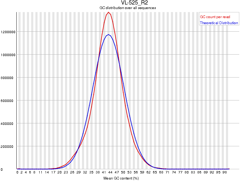
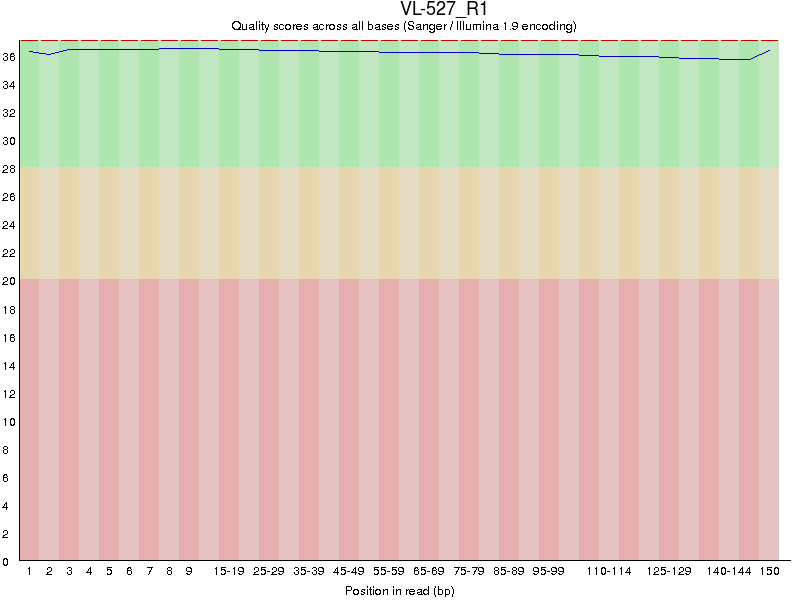
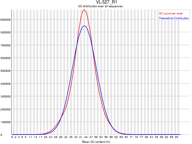
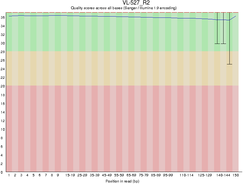
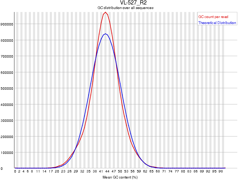
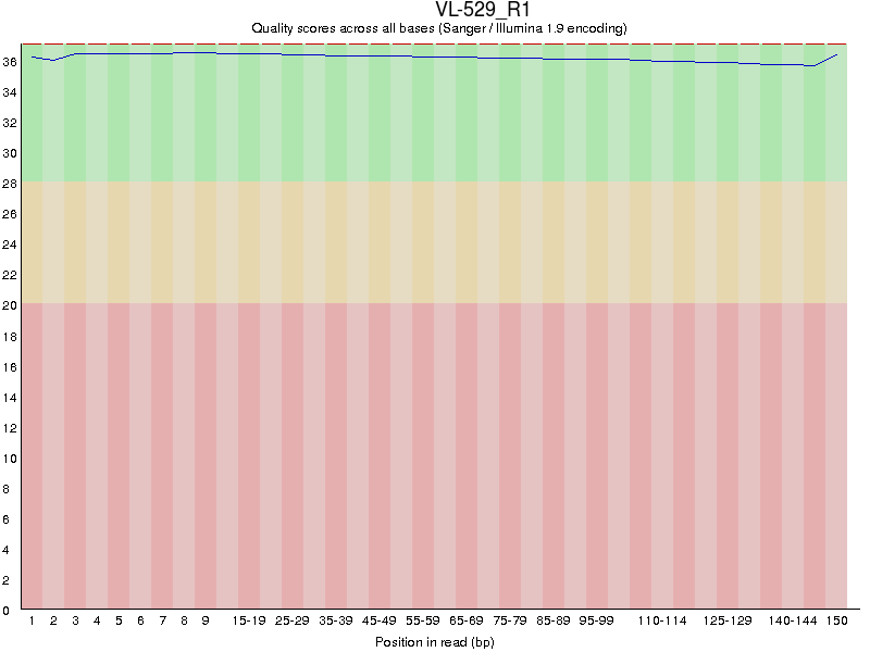
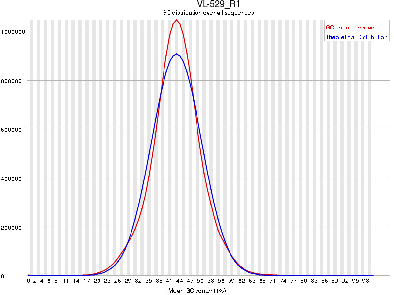
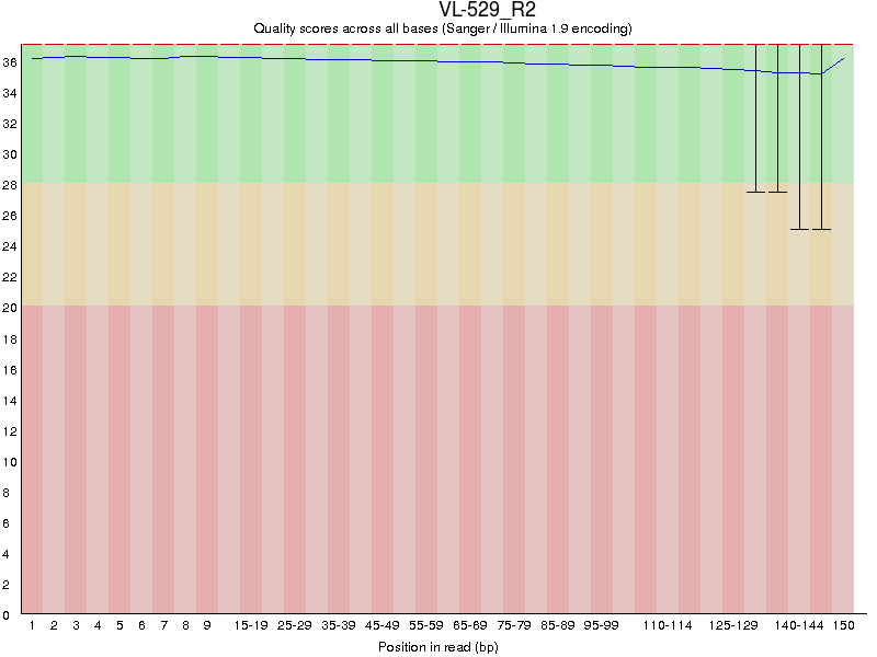
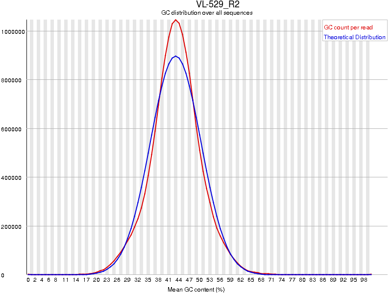
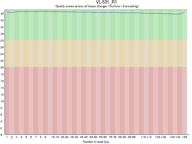
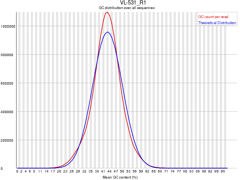
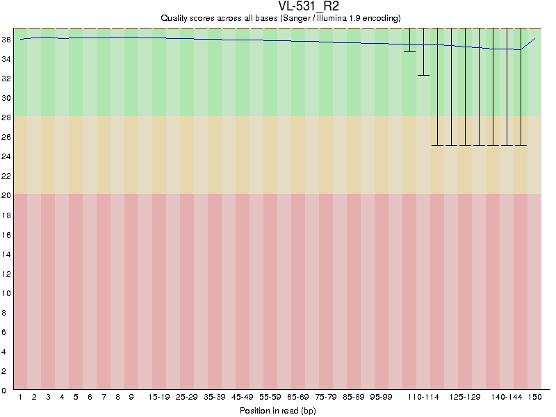
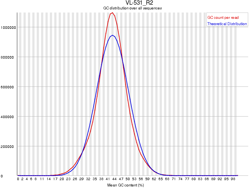
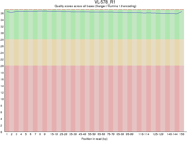
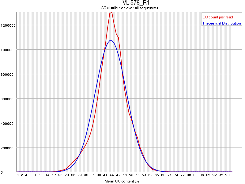
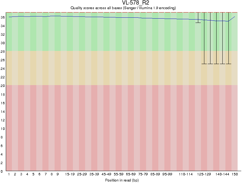
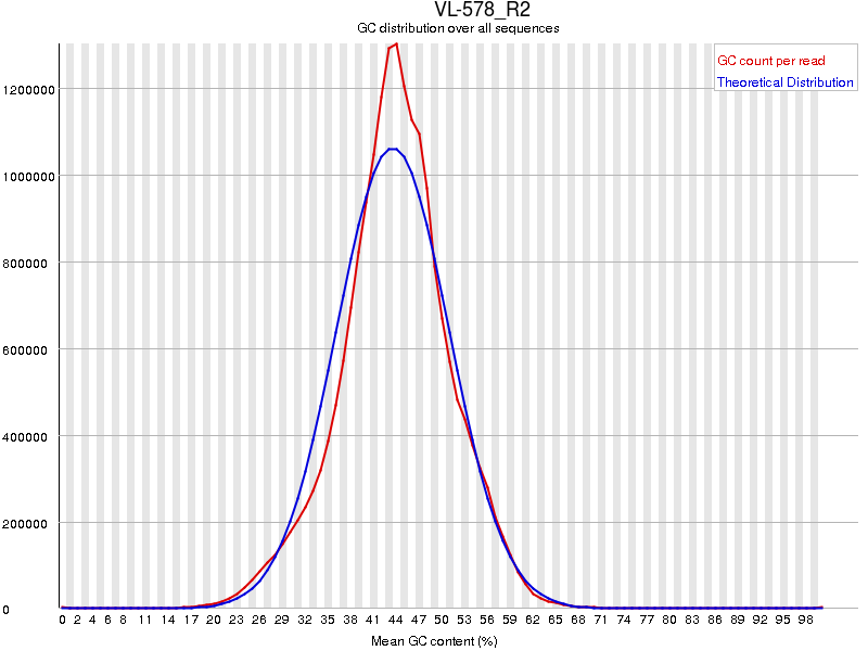
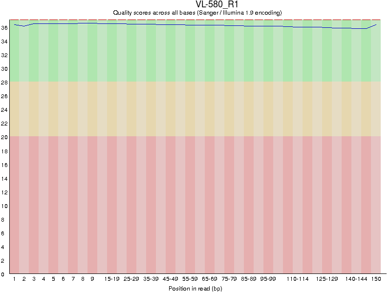
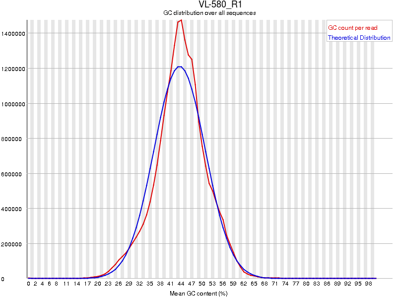
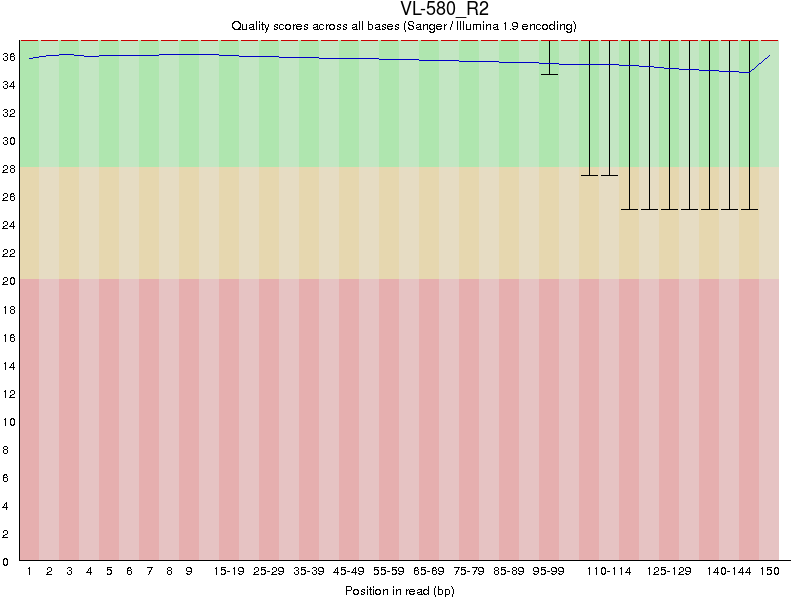
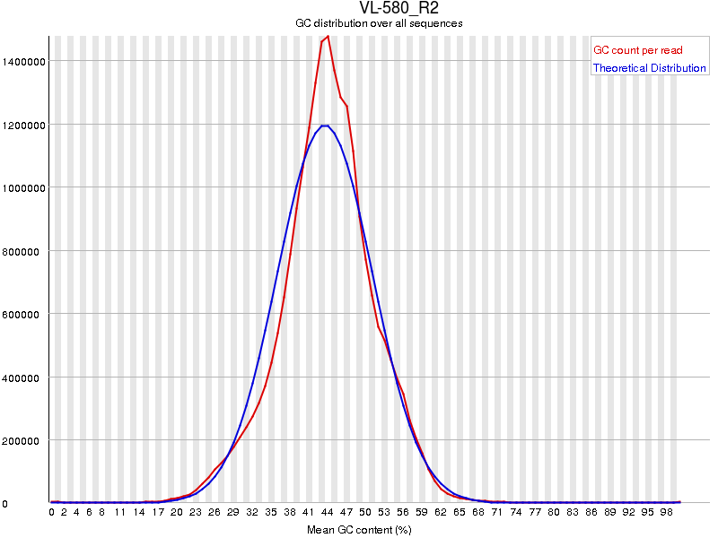
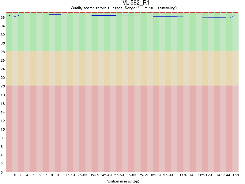
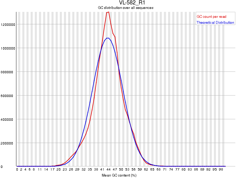
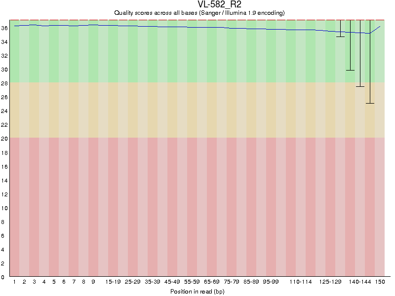
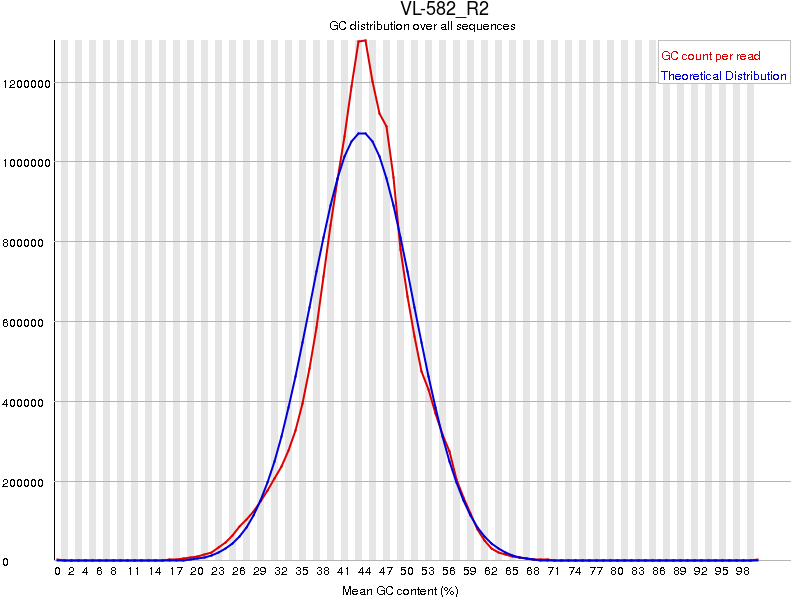
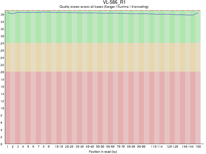
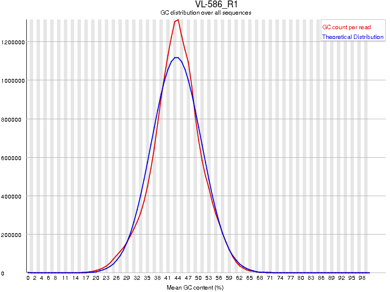
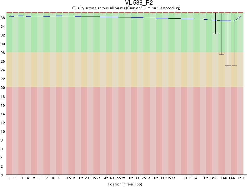
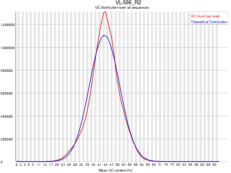
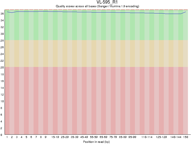
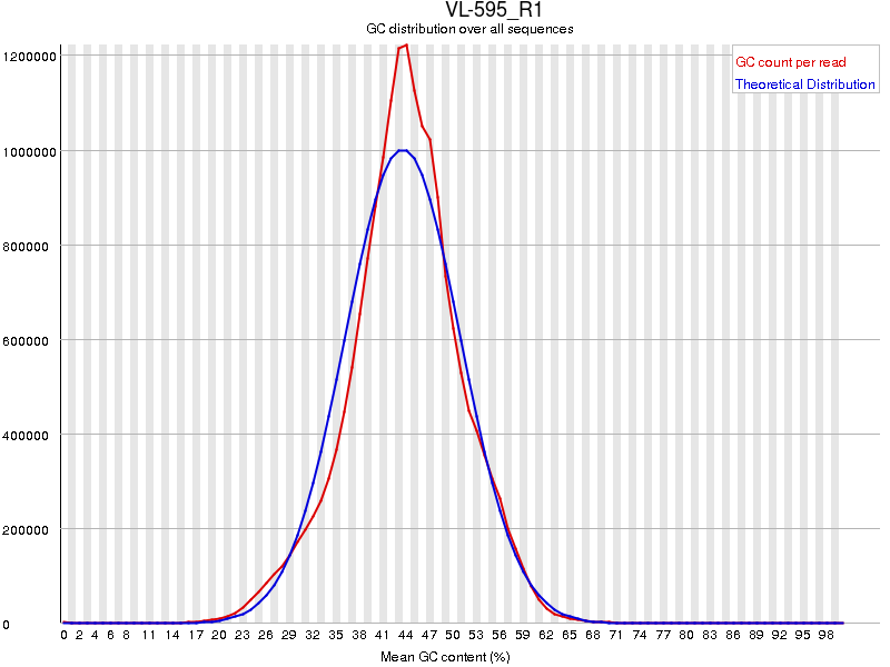
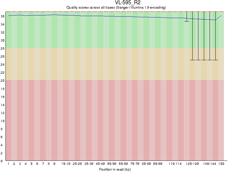
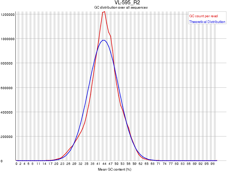
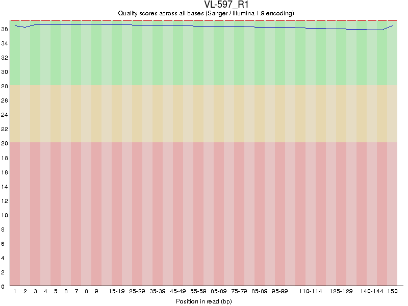
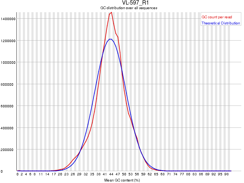
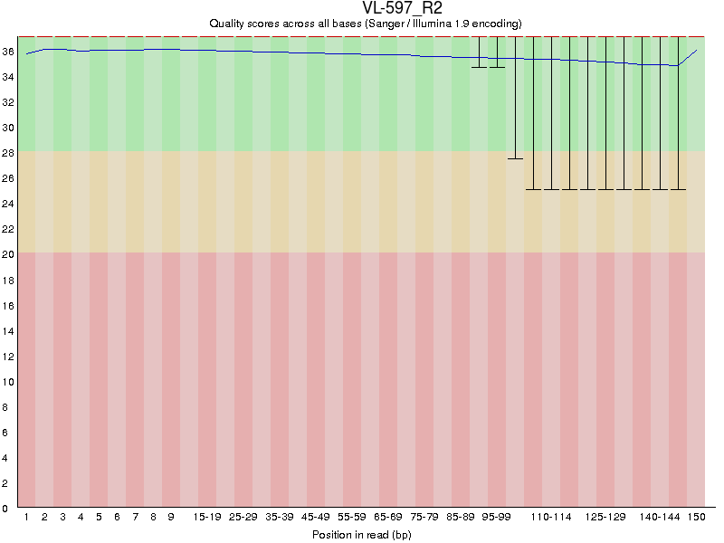
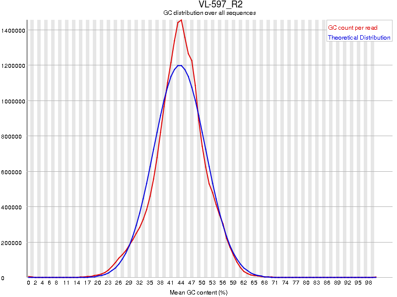
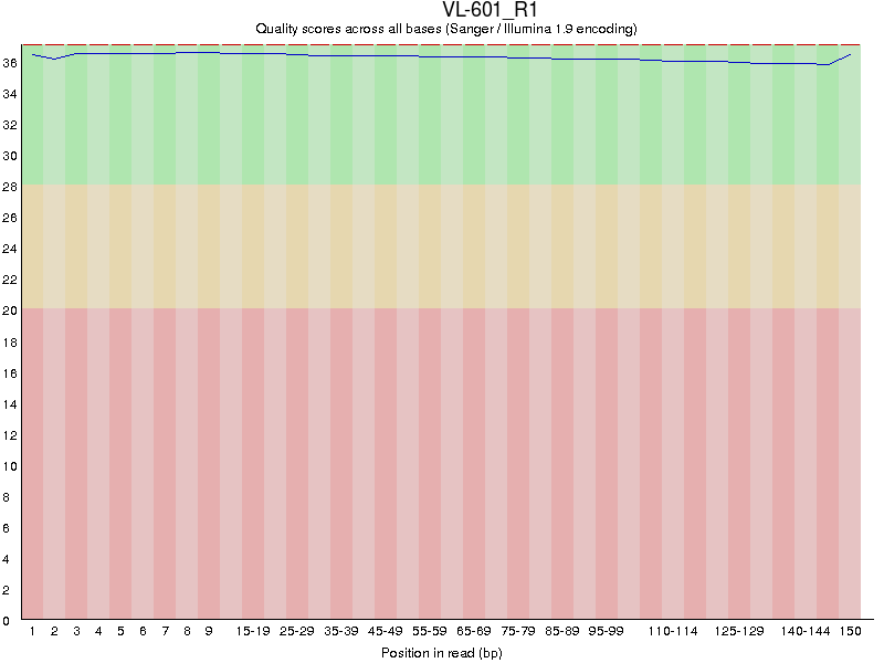
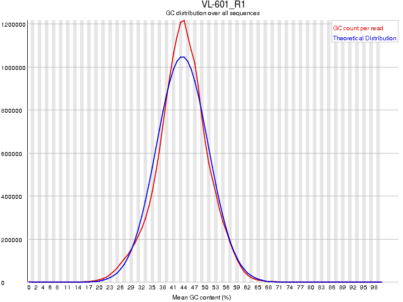
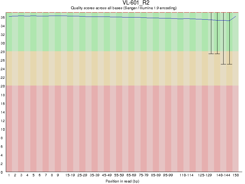
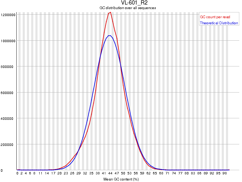
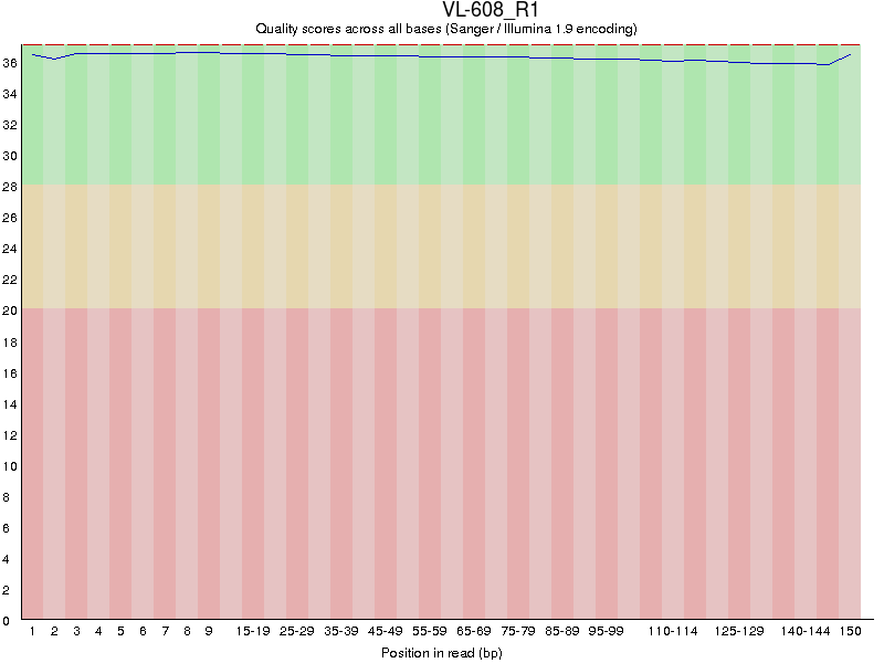
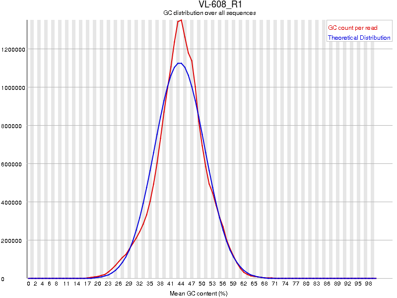
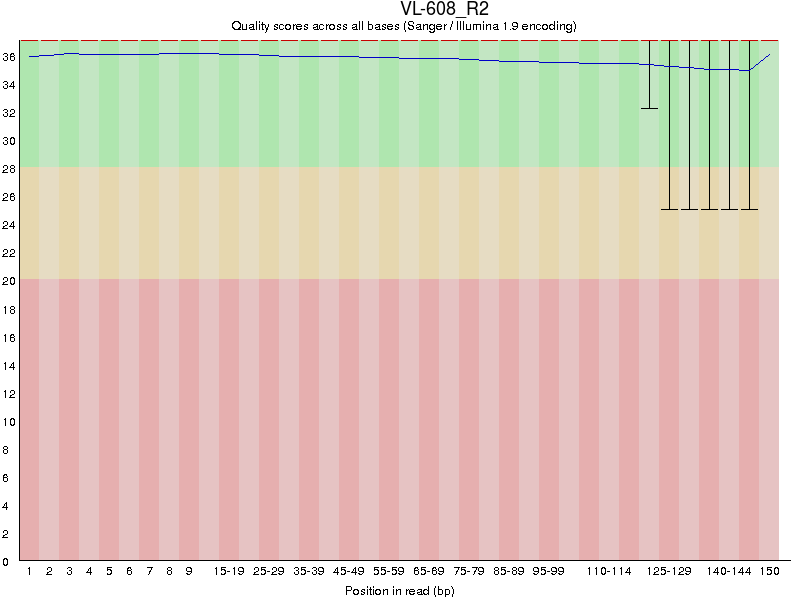
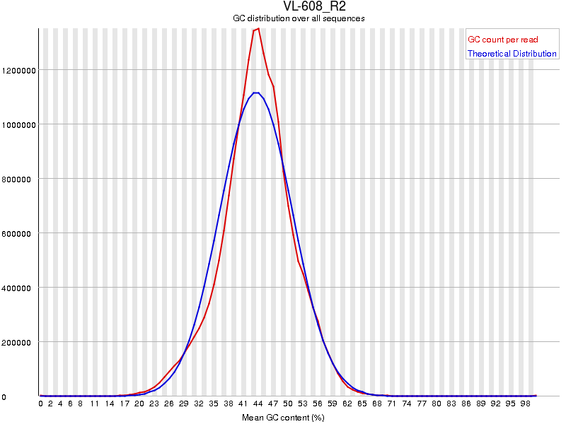
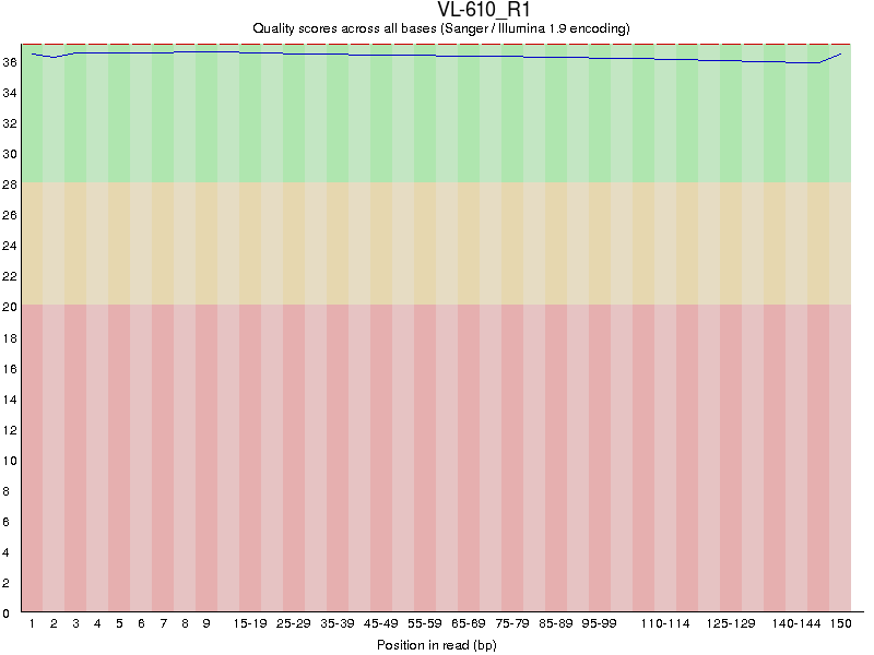
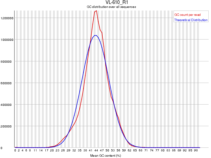
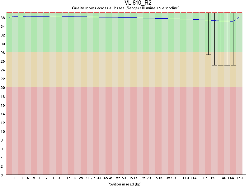
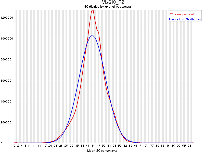
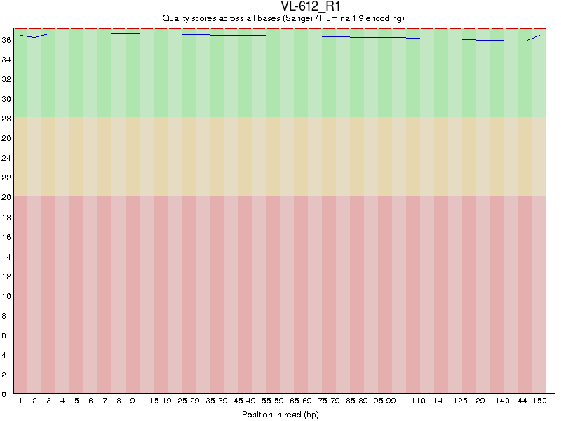
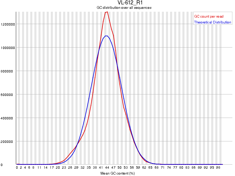
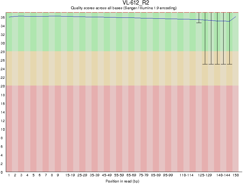
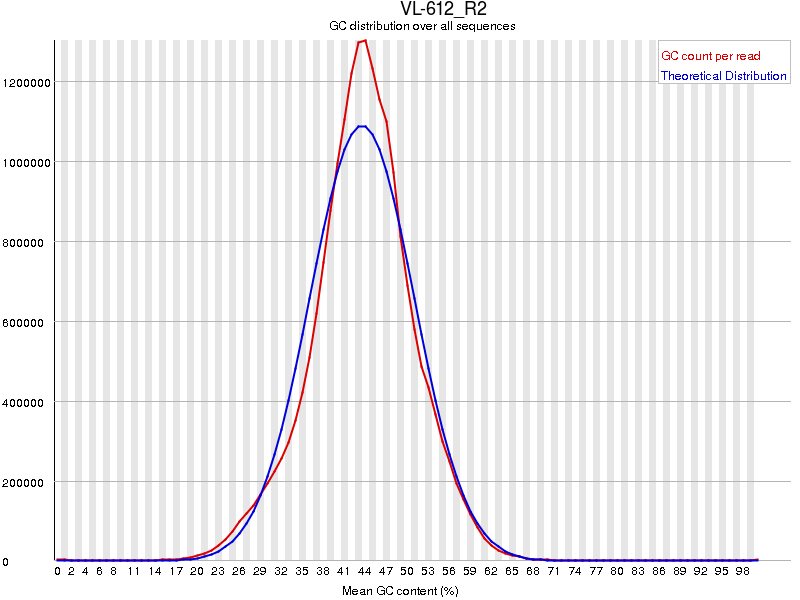
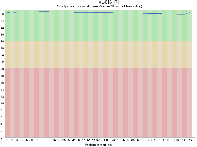
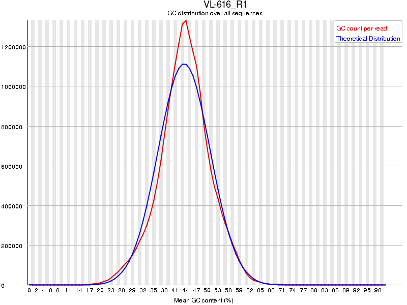
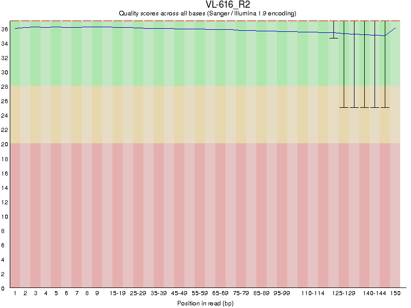
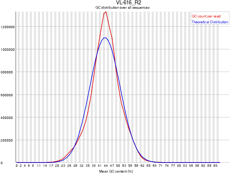
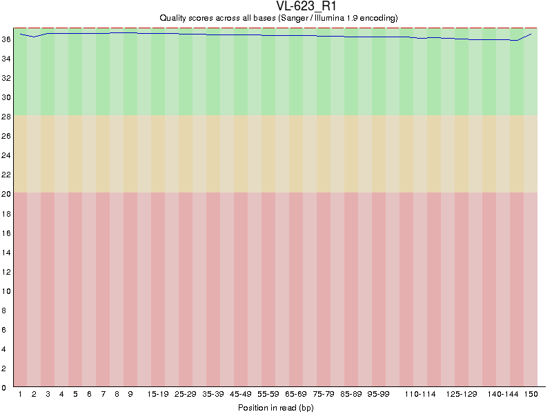
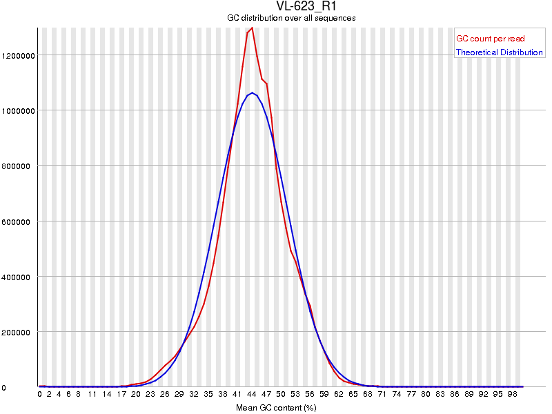
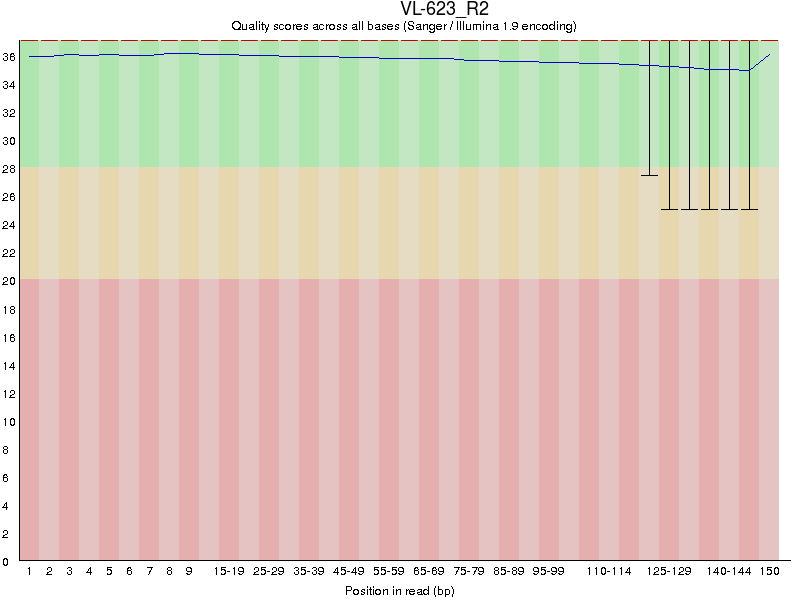
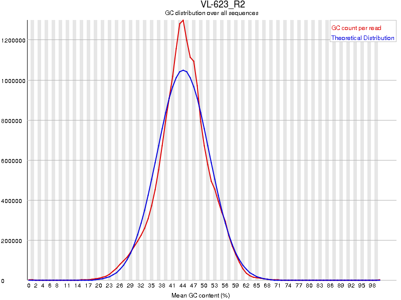
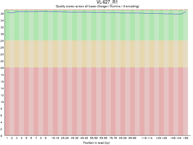
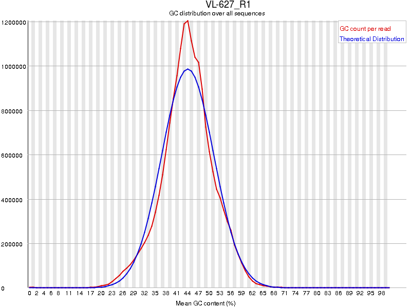
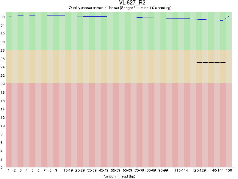
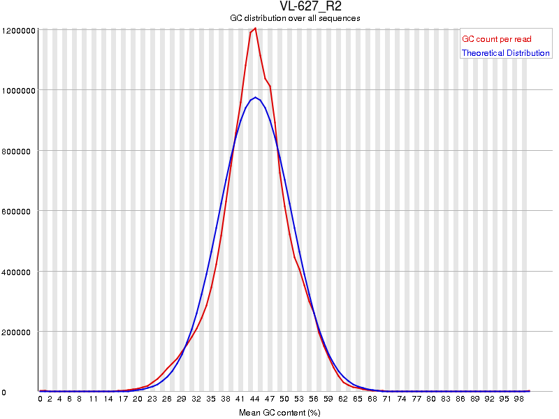
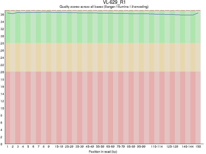
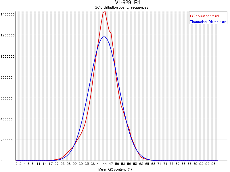
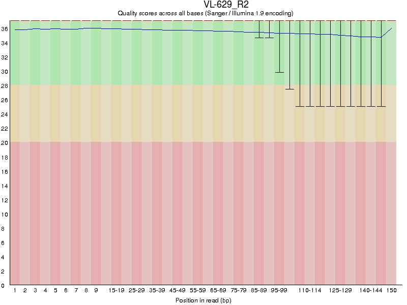
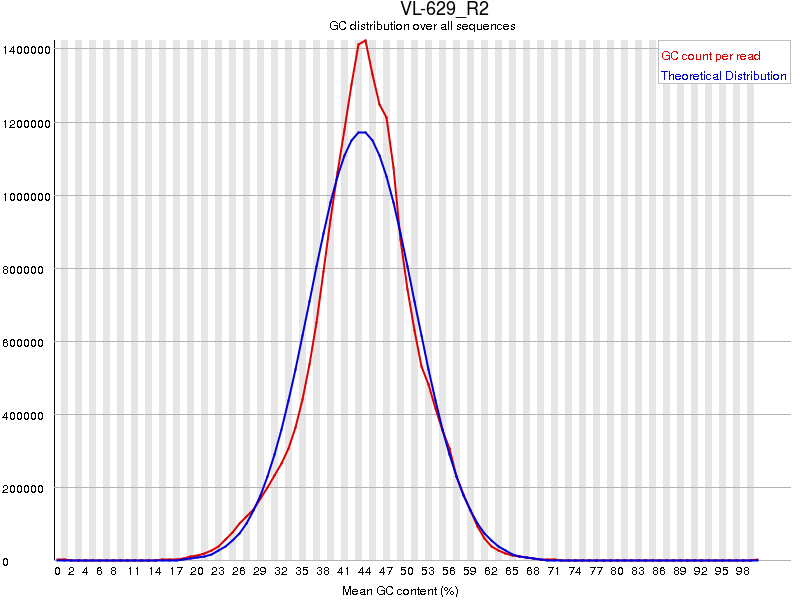
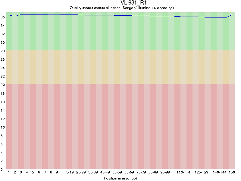
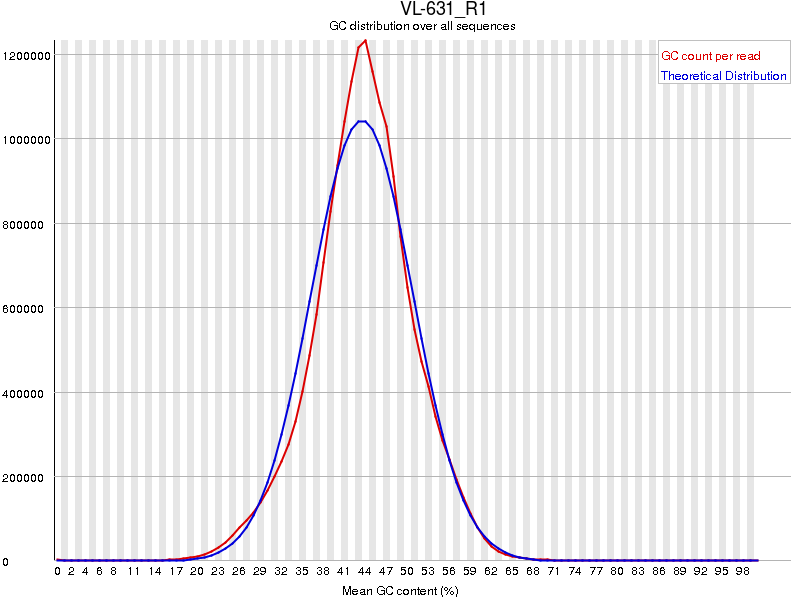
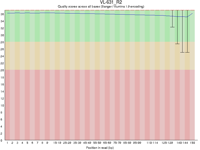
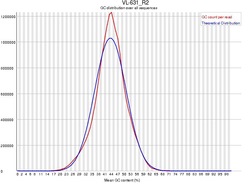
Sequence reads were trimmed to remove possible adapter sequences and nucleotides with poor quality using Trimmomatic v.0.36. The trimmed reads were mapped to the Pisum_sativum reference genome available on ENSEMBL using the STAR aligner v.2.5.2b. The STAR aligner is a splice aligner that detects splice junctions and incorporates them to help align the entire read sequences. BAM files were generated as a result of this step. Below are the statistics of mapping the reads to the reference genome.
Code
#pkg library(tidyverse)library(patchwork)library(readxl)# srcsource(here::here("src/function/stat_function/stat_analysis_main.R")) # for make plot source(here::here("src/function/fig_export.R")) # This function saves a given plot (plot_x) as both a PDF and a high-resolution PNG file at specified dimensions.# cosmeticspallet=read_excel(here::here("data/color_palette.xlsm")) %>%filter(set =="edaphic_condition") %>% dplyr::select(color, treatment) %>%pull(color) %>%setNames(read_excel(here::here("data/color_palette.xlsm")) %>%filter(set =="edaphic_condition") %>%pull(treatment) )
Unique gene hit counts were calculated by using featureCounts from the Subread package v.1.5.2. The hit counts were summarized and reported using the gene_id feature in the annotation file. Only unique reads that fell within exon regions were counted.
Source Code
---output: html_documenteditor_options: chunk_output_type: console---## Intro RNAseq {#sec-rnaseq}::: {.callout-caution}## To be done before publication- [ ] Write results article- [ ] Publish raw data from rnaseq- [x] Clean the code- [ ] Share the code to git:::## Project summary- Customer Karine GALLARDO- Email karine.gallardo-guerrero@inrae.fr- Sample Type human RNA- Application mRNA sequencing via polyA selection- Quote Number 50-595289658- Configuration HiSeq 2x150bp HiSeq 2x150bp## Description of workflow### RNA-seq Library Prepraration Workflow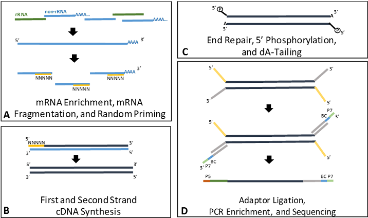{fig-align="center"}### Bioinformatics Analysis Workflow.png){fig-align="center"}## Mapping sequence reads to the reference genomeSequence reads were trimmed to remove possible adapter sequences and nucleotides with poor quality using Trimmomatic v.0.36. The trimmed reads were mapped to the Pisum_sativum reference genome available on ENSEMBL using the STAR aligner v.2.5.2b. The STAR aligner is a splice aligner that detects splice junctions and incorporates them to help align the entire read sequences. BAM files were generated as a result of this step. Below are the statistics of mapping the reads to the reference genome.```{r}#pkg library(tidyverse)library(patchwork)library(readxl)# srcsource(here::here("src/function/stat_function/stat_analysis_main.R")) # for make plot source(here::here("src/function/fig_export.R")) # This function saves a given plot (plot_x) as both a PDF and a high-resolution PNG file at specified dimensions.# cosmeticspallet=read_excel(here::here("data/color_palette.xlsm")) %>%filter(set =="edaphic_condition") %>% dplyr::select(color, treatment) %>%pull(color) %>%setNames(read_excel(here::here("data/color_palette.xlsm")) %>%filter(set =="edaphic_condition") %>%pull(treatment) )``````{r, ResultMatchGenomeReference, eval=F}sample_info<-read_excel(here::here("data/rnaseq/50-595289658_NGSBI_Completed_file_send to GENEWIZ_2021-12-22.xlsx"), sheet = "Groupings", skip = 2) %>% filter(!`Sample Name` %in% c("Vegetative leaves", "Roots")) %>% dplyr::rename(sample_id = "Sample Name", group = "Groupings (i.e. biological replicates)") %>% dplyr::select(sample_id, group) %>% tidyr::separate(group, into = c("compartment", "sampling", "genotype", "water_condition", "sulfur_condition"), sep = "_") %>% dplyr::mutate(genotype = case_when( genotype %in% "2684" ~ "W78*", genotype %in% "4693" ~ "E568K", genotype %in% "CAM2684" ~ "WT1", genotype %in% "CAM4693" ~ "WT2", genotype %in% "KAY" ~ "KAY"), genotype = forcats::fct_relevel(genotype, "KAY", "WT1", "W78*", "WT2", "E568K"), water_condition = forcats::fct_relevel(water_condition, "WW", "WS"), condition = paste(sep = "_", genotype, sulfur_condition), sulfur_condition = forcats::fct_relevel(sulfur_condition, "SS", "SD"), sampling = forcats::fct_relevel(sampling, "E0", "E1", "E2"), edaphic_condition = paste(sep = "_", water_condition, sulfur_condition), edaphic_condition = forcats::fct_relevel(edaphic_condition, "WW_SS", "WW_SD", "WS_SS", "WS_SD") )mapping_resum_r<- read_csv(file = here::here("data/rnaseq/AZENTA RNA-Seq Analysis Report.csv"), show_col_types = FALSE) %>% dplyr::rename(c("Unique_mapped_reads" = `% Unique Mapped Reads` , "Total_reads" = `Total Reads`, "sample_id" = `Sample ID`)) %>% left_join(., sample_info, by = "sample_id") %>% filter(compartment == "R") %>% as.data.frame()mapping_resum_vl<- read_csv(file = here::here("data/rnaseq/AZENTA RNA-Seq Analysis Report.csv"), show_col_types = FALSE) %>% dplyr::rename(c("Unique_mapped_reads" = `% Unique Mapped Reads` , "Total_reads" = `Total Reads`, "sample_id" = `Sample ID`)) %>% left_join(., sample_info, by = "sample_id") %>% filter(compartment == "VL") %>% as.data.frame()plot_unique_r=stat_analyse( data=mapping_resum_r, column_value = "Unique_mapped_reads", category_variables = c("edaphic_condition"), grp_var = "genotype", show_plot = T, outlier_show = T, label_outlier = "sample_id", biologist_stats = T, Ylab_i = paste0("Unique Mapped Reads for root"), control_conditions = c("WW_SS"), hex_pallet = pallet, strip_normale = F)plot_unique_vl=stat_analyse( data=mapping_resum_vl, column_value = "Unique_mapped_reads", category_variables = c("edaphic_condition"), grp_var = "genotype", show_plot = T, outlier_show = T, label_outlier = "sample_id", biologist_stats = T, Ylab_i = paste0("Unique Mapped Reads for vegetative leaves"), control_conditions = c("WW_SS"), hex_pallet = pallet, strip_normale = F)plot_total_r=stat_analyse( data=mapping_resum_r, column_value = "Total_reads", category_variables = "edaphic_condition", grp_var = "genotype", show_plot = T, outlier_show = T, label_outlier = "sample_id", biologist_stats = T, Ylab_i = paste0("Total Mapped Reads for root"), control_conditions = c("WW_SS"), hex_pallet = pallet, strip_normale = F)plot_total_vl=stat_analyse( data=mapping_resum_vl, column_value = "Total_reads", category_variables = "edaphic_condition", grp_var = "genotype", show_plot = T, outlier_show = T, label_outlier = "sample_id", biologist_stats = T, Ylab_i = paste0("Total Mapped Reads for vegetative leaves"), control_conditions = c("WW_SS"), hex_pallet = pallet, strip_normale = F)plot_unique_r = plot_unique_r[["plot"]]+labs(color="Treatment",fill="Treatment")plot_unique_vl = plot_unique_vl[["plot"]]+labs(color="Treatment",fill="Treatment")plot_total_r = plot_total_r[["plot"]]+labs(color="Treatment",fill="Treatment")plot_total_vl = plot_total_vl[["plot"]]+labs(color="Treatment",fill="Treatment") px=(plot_unique_r + plot_unique_vl) / (plot_total_r + plot_total_vl) + plot_layout(guides = "collect") & theme(legend.position = "bottom")#export to deletfig_export(path = here::here("report/rnaseq/plot/mapped_reads_performance"), px, height = 10, width = 12)```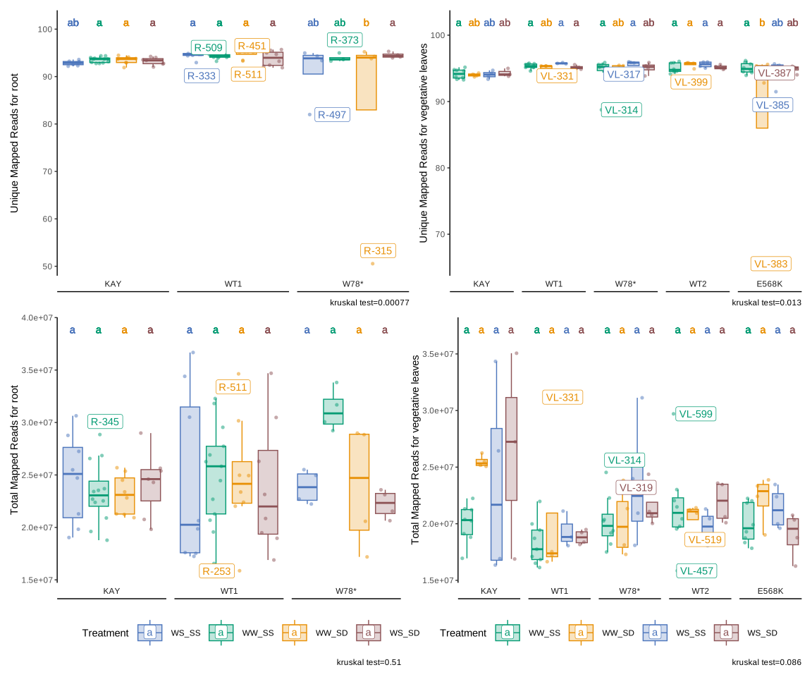{fig-align="center"}```{r, echo=FALSE, results = "asis"}# function remove_terms <- function(text_vec, terms_vec, ignore_case = TRUE) { # Construit une regex du type "\\b(terme1|terme2|terme3)\\b" pattern <- paste0("\\b(", paste(terms_vec, collapse = "|"), ")\\b") text_vec %>% str_remove_all(regex(pattern, ignore_case = ignore_case)) %>% str_squish() # retire les espaces multiples laissés par la suppression}word_to_del <- c("seed_", "reproductive leaf_", "vegetative leaf_")image_files <- list.files("img/fastqc/", pattern = "\\.png$", full.names = TRUE)# Extraire le nom des fichiers sans extensionimage_names <- tools::file_path_sans_ext(basename(image_files))# Extraire la première et la deuxième valeur séparées par "_"first_values <- sapply(strsplit(image_names, "_"), function(x) x[1])second_values <- sapply(strsplit(image_names, "_"), function(x) x[2])# Identifier les groupes uniques pour la première valeurunique_first <- unique(first_values)# Création du code pour le panel-tabset globaltabset_code <- ":::: {.panel-tabset}\n"# Pour chaque groupe du premier niveaufor (grp1 in unique_first) { tabset_code <- paste0(tabset_code, "## ", grp1, "\n\n", ":::: {.panel-tabset}\n") # Indices des images appartenant à ce groupe indices_first <- which(first_values == grp1) # Identifier les sous-groupes (deuxième valeur) dans ce groupe unique_second <- unique(second_values[indices_first]) # Pour chaque sous-groupe du deuxième niveau for (grp2 in unique_second) { tabset_code <- paste0(tabset_code, "### ", grp2, "\n\n", ":::: {.panel-tabset}\n") # Sélectionner les images correspondant à ce sous-groupe indices_second <- indices_first[second_values[indices_first] == grp2] for (i in indices_second) { tabset_code <- paste0(tabset_code, "#### ", remove_terms(image_names[i], word_to_del), "\n\n", " } tabset_code <- paste0(tabset_code, "::::\n\n") # fermeture du sous-tabset du deuxième niveau } tabset_code <- paste0(tabset_code, "::::\n\n") # fermeture du sous-tabset du premier niveau}tabset_code <- paste0(tabset_code, "::::")cat(tabset_code)```## Extracting gene hit countsUnique gene hit counts were calculated by using featureCounts from the Subread package v.1.5.2. The hit counts were summarized and reported using the gene_id feature in the annotation file. Only unique reads that fell within exon regions were counted.

.png)