After extraction of gene hit counts, the gene hit counts table was used for downstream differential expression analysis. Using DESeq2, a comparison of gene expression between the customer-defined groups of samples was performed. The Wald test was used to generate p-values and log2 fold changes. Genes with an adjusted p-value < 0.05 and absolute log2 fold change > 1 were called as differentially expressed genes for each comparison. Below are the results of the diferential gene expression analyses for all comparisons provided.
Be careful, there are probably genotyping errors for the mutants.
To be reviewed with Karine and Marion
Code
# pkglibrary(dplyr)library(factoextra)library(DESeq2) # BiocManager::install("DESeq2")library(readxl)library(tidyr)library(vsn) # for meanSdPlot #BiocManager::install("vsn")library(pheatmap)library(RColorBrewer)library(ggrepel)library(readxl)library(gridExtra)library(patchwork)library(ggrepel)library(mixOmics)# srcsource(here::here("src/function/stat_function/stat_analysis_main.R")) # for make plot source(here::here("src/function/fig_export.R")) # This function saves a given plot (plot_x) as both a PDF and a high-resolution PNG file at specified dimensions.# cosmeticspallet=read_excel(here::here("data/color_palette.xlsm")) %>%filter(set =="edaphic_condition") %>% dplyr::select(color, treatment) %>%pull(color) %>%setNames(read_excel(here::here("data/color_palette.xlsm")) %>%filter(set =="edaphic_condition") %>%pull(treatment) )
7.1 Data importation
Read Counting: Ensure that your count table includes counts. Your count table should have rows for each gene and columns for each sample.
Create a DESeqDataSet object using the count data, specifying the experimental design and sample information. I need to create a table that summarizes all my conditions (water stress, heat stress, genotype). In my case I have a three factor experiment
Code
sample_list_rnaseq <-read_excel(here::here("data/rnaseq/50-595289658_NGSBI_Completed_file_send to GENEWIZ_2021-12-22.xlsx"), sheet ="Groupings", skip =2) %>%filter(!`Sample Name`%in%c("Vegetative leaves", "Roots")) %>% dplyr::rename(sample_id ="Sample Name", group ="Groupings (i.e. biological replicates)") %>% dplyr::select(sample_id, group) %>% tidyr::separate(group, into =c("compartment", "sampling", "genotype", "water_condition", "sulfur_condition"), sep ="_") %>% dplyr::mutate(genotype =case_when( genotype %in%"2684"~"W78*", genotype %in%"4693"~"E568K", genotype %in%"CAM2684"~"WT1", genotype %in%"CAM4693"~"WT2", genotype %in%"KAY"~"KAY"),genotype = forcats::fct_relevel(genotype, "KAY", "WT1", "W78*", "WT2", "E568K"),water_condition = forcats::fct_relevel(water_condition, "WW", "WS"),condition =paste(sep ="_", genotype, water_condition, sulfur_condition), sulfur_condition = forcats::fct_relevel(sulfur_condition, "SS", "SD"),sampling = forcats::fct_relevel(sampling, "E0", "E1", "E2"),edaphic_condition =paste(sep ="_", water_condition, sulfur_condition), edaphic_condition = forcats::fct_relevel(edaphic_condition, "WW_SS", "WW_SD", "WS_SS", "WS_SD"),compartment = forcats::fct_relevel(compartment, "VL", "R") )# root_sample_list_rnaseq <-read_excel(here::here("data/rnaseq/AZENTA RNA-Seq Analysis Report mapping sequence reads to the reference genome.xlsx")) %>%# mutate(sample=gsub("-",".",`Sample ID`)) %>%# dplyr::select(sample,genotype,water_condition,heat_condition) %>%# mutate(id_azenta=sample) %>% # drop_na(sample) %>% # column_to_rownames("id_azenta") %>% # mutate_all(list(as.factor))write_csv(file = here::here("data/rnaseq/output/sample_list_rnaseq.csv"), sample_list_rnaseq)# show table# 1. Helper that does the "long → wide" reshapingclean_tbl <- sample_list_rnaseq %>%# 1. collapse all samples that share compartment, sampling & genotype,# ignoring water/sulfur differencesgroup_by(compartment, sampling,water_condition, sulfur_condition, genotype) %>%summarise(sample_id =paste(sample_id, collapse =", "),.groups ="drop") %>%# 2. reshape so genotypes become the columnspivot_wider(id_cols =c(compartment, sampling, water_condition, sulfur_condition), # ← *only* these two define the rowsnames_from = genotype,values_from = sample_id ) %>%# 3. keep desired genotype orderrelocate(KAY, .after =last_col()) %>%# easiest way to push KAY to the endarrange(compartment, sampling, water_condition, sulfur_condition)knitr::kable(clean_tbl,caption ="Samples per compartment × sampling; cells list sample IDs")
Samples per compartment × sampling; cells list sample IDs
compartment
sampling
water_condition
sulfur_condition
WT1
W78*
WT2
E568K
KAY
VL
E0
WW
SS
VL-582, VL-597, VL-612, VL-627
VL-578, VL-593, VL-608, VL-623
VL-584, VL-599, VL-614, VL-629
VL-580, VL-595, VL-610, VL-625
VL-586, VL-601, VL-616, VL-631
VL
E1
WW
SS
VL-329, VL-389, VL-449, VL-509, VL-313
VL-373, VL-433, VL-493, VL-314
VL-337, VL-397, VL-457, VL-517
VL-321, VL-381, VL-441, VL-501
VL-345, VL-405, VL-465, VL-525
VL
E1
WW
SD
VL-331, VL-391, VL-451, VL-511
VL-315, VL-375, VL-435, VL-495
VL-339, VL-399, VL-459, VL-519
VL-323, VL-383, VL-443, VL-503
VL-347, VL-407, VL-467, VL-527
VL
E1
WS
SS
VL-333, VL-393, VL-513
VL-317, VL-377, VL-437, VL-497
VL-341, VL-401, VL-461, VL-521
VL-325, VL-385, VL-445, VL-505
VL-349, VL-409, VL-469, VL-529
VL
E1
WS
SD
VL-395, VL-455, VL-515, VL-335
VL-319, VL-379, VL-439, VL-499
VL-343, VL-403, VL-463, VL-523
VL-327, VL-387, VL-447, VL-507
VL-351, VL-411, VL-531
R
E0
WW
SS
R-582, R-597, R-612, R-627
NA
NA
NA
R-586, R-601, R-616, R-631
R
E1
WW
SS
R-329, R-389, R-449, R-509, R-313
R-373, R-433, R-493, R-314
NA
NA
R-345, R-405, R-465, R-525
R
E1
WW
SD
R-331, R-391, R-451, R-511
R-315, R-375, R-435, R-495
NA
NA
R-347, R-407, R-467, R-527
R
E1
WS
SS
R-333, R-393, R-513
R-317, R-377, R-437, R-497
NA
NA
R-349, R-409, R-469, R-529
R
E1
WS
SD
R-455, R-515, R-335
R-319, R-379, R-439, R-499
NA
NA
R-351, R-411, R-531
R
E2
WW
SS
R-143, R-179, R-251, R-221
NA
NA
NA
R-151, R-187, R-259, R-223
R
E2
WW
SD
R-145, R-181, R-216, R-253
NA
NA
NA
R-153, R-189, R-224, R-261
R
E2
WS
SS
R-147, R-183, R-218, R-255, R-139
NA
NA
NA
R-155, R-226, R-263, R-192
R
E2
WS
SD
R-149, R-185, R-220, R-257, R-178
NA
NA
NA
R-157, R-193, R-227, R-265
7.2 Filtering and normalization of low-count genes
Use DESeq2’s normalization functions to normalize the count data.
I decided to analyze the data without using the exogenous spike-ins for normalization.So i remove the spike-ins genes (i.e begin by ERCC)
7.3 Pre-filtering and normalize for full analyse
While it is not necessary to pre-filter low count genes before running the DESeq2 functions, there are two reasons which make pre-filtering useful: by removing rows in which there are very few reads, we reduce the memory size of the dds data object, and we increase the speed of the transformation and testing functions within DESeq2.
Using vst() or varianceStabilizingTransformation() ? This is a wrapper for the varianceStabilizingTransformation (VST) that provides much faster estimation of the dispersion trend used to determine the formula for the VST. The speed-up is accomplished by subsetting to a smaller number of genes in order to estimate this dispersion trend. The subset of genes is chosen deterministically, to span the range of genes’ mean normalized count. This wrapper for the VST is not blind to the experimental design: the sample covariate information is used to estimate the global trend of genes’ dispersion values over the genes’ mean normalized count. It can be made strictly blind to experimental design by first assigning a design of ~1 before running this function, or by avoiding subsetting and using varianceStabilizingTransformation.
This function calculates a variance stabilizing transformation (VST) from the fitted dispersion-mean relation(s) and then transforms the count data (normalized by division by the size factors or normalization factors), yielding a matrix of values which are now approximately homoskedastic (having constant variance along the range of mean values). The transformation also normalizes with respect to library size. The rlog is less sensitive to size factors, which can be an issue when size factors vary widely. These transformations are useful when checking for outliers or as input for machine learning techniques such as clustering or linear discriminant analysis.
Change level to adapte deseq (control is WT and OT for (Well watered and Optimal sulfure condition) )
full dataset to (root and vegetative leaves (VL)) to compare the influence of the stress depending of the type of sampling and genotype. VL are more sensible to stress ?. I can do that only at E1 and only for WT1 (Caméor) and KAY (Kayane).
Code
df_count <-read_csv(file = here::here("data/rnaseq/raw_counts.csv"), show_col_types =FALSE) %>% dplyr::rename(psat =1) %>%column_to_rownames("psat")sample_list_rnaseq <-read_csv(file = here::here("data/rnaseq/output/sample_list_rnaseq.csv"),show_col_types =FALSE) %>% dplyr::mutate(genotype = forcats::fct_relevel(genotype, "KAY", "WT1", "W78*", "WT2", "E568K"),water_condition = forcats::fct_relevel(water_condition, "WW", "WS"),sulfur_condition = forcats::fct_relevel(sulfur_condition, "SS", "SD"),sampling = forcats::fct_relevel(sampling, "E0", "E1", "E2"),edaphic_condition = forcats::fct_relevel(edaphic_condition, "WW_SS", "WW_SD", "WS_SS", "WS_SD"),compartment = forcats::fct_relevel(compartment, "VL", "R"), condition = forcats::fct_relevel(condition, "KAY_WW_SS", "KAY_WW_SD", "KAY_WS_SS", "KAY_WS_SD","WT1_WW_SS", "WT1_WW_SD", "WT1_WS_SS", "WT1_WS_SD","W78*_WW_SS", "W78*_WW_SD", "W78*_WS_SS", "W78*_WS_SD","WT2_WW_SS", "WT2_WW_SD", "WT2_WS_SS", "WT2_WS_SD","E568K_WW_SS","E568K_WW_SD", "E568K_WS_SS", "E568K_WS_SD" ) )## 0. Make sure the *columns* of the count matrix are exactly## the samples you keep in your metadata ------------------sample_list_rnaseq_full <- sample_list_rnaseq### filtercount_table_full<-df_count %>% dplyr::select(sample_list_rnaseq_full$sample_id)# ## 1. Prefilter: keep genes with ≥10 counts in ≥90 % of samples ----------# keep <- rowSums(count_table_vl >= 10) >= 0.9 * ncol(count_table_vl)# count_table_vl_filt <- count_table_vl[keep, ]# ## 1. Prefilter: Keep a gene if it has ≥ 10 raw counts in at least min_samples libraries within any one experimental group.group <-with(sample_list_rnaseq_full, # metadata tibbleinteraction(compartment, sampling, genotype, water_condition, sulfur_condition,drop =TRUE)) # drop unused levels## 1B Apply the filtermin_count <-10# threshold on raw countsmin_samples <-3# ≥ this many libraries in the same groupkeep_manual <-apply(count_table_full, 1, function(cnts) {# cnts = vector of counts for ONE gene across all samples hits_per_group <-tapply(cnts >= min_count, group, sum)max(hits_per_group) >= min_samples})sum(keep_manual) # how many genes survive?count_table_filt <- count_table_full[keep_manual, ]## 2. Build DESeqDataSet and run DESeq -------------------------------### deseqdds_full <-DESeqDataSetFromMatrix(countData = count_table_filt,colData=sample_list_rnaseq_full,design =~compartment+sampling+genotype+water_condition+sulfur_condition+genotype:water_condition+genotype:sulfur_condition+water_condition:sulfur_condition+genotype:water_condition:sulfur_condition)dds_full_1 <-DESeq(dds_full)# see https://www.biostars.org/p/9573278/ for spike-ins normalization# Change control conditiondds_full_1$water_condition =relevel(dds_full_1$water_condition, "WW")dds_full_1$sulfur_condition =relevel(dds_full_1$sulfur_condition, "SS")## 3. Transformations for visualisation -------------------------------rld_full <-rlog(dds_full_1, blind =TRUE)vst_full <-vst(dds_full_1, blind =TRUE)# all the info of the dds filter resultsNames(dds_full_1)colData(dds_full_1) # to know metadatadesign(dds_full_1)################## comparison VL to Root at E1 without stress condition ####################################################################### 0. Make sure the *columns* of the count matrix are exactly## the samples you keep in your metadata ------------------sample_list_rnaseq_comparison_compartment_E1_WW_SS <- sample_list_rnaseq %>%filter(sampling =="E1", genotype %in%c("WT1", "KAY"), edaphic_condition =="WW_SS" )### filtercount_table_comparison_compartment_E1_WW_SS<-df_count %>% dplyr::select(sample_list_rnaseq_comparison_compartment_E1_WW_SS$sample_id)# ## 1. Prefilter: keep genes with ≥10 counts in ≥90 % of samples ----------# keep <- rowSums(count_table_vl >= 10) >= 0.9 * ncol(count_table_vl)# count_table_vl_filt <- count_table_vl[keep, ]# ## 1. Prefilter: Keep a gene if it has ≥ 10 raw counts in at least min_samples libraries within any one experimental group.group <-with(sample_list_rnaseq_comparison_compartment_E1_WW_SS, # metadata tibbleinteraction(compartment, genotype,drop =TRUE)) # drop unused levels## 1B Apply the filtermin_count <-10# threshold on raw countsmin_samples <-3# ≥ this many libraries in the same groupkeep_manual <-apply(count_table_comparison_compartment_E1_WW_SS, 1, function(cnts) {# cnts = vector of counts for ONE gene across all samples hits_per_group <-tapply(cnts >= min_count, group, sum)max(hits_per_group) >= min_samples})sum(keep_manual) # how many genes survive?count_table_filt <- count_table_comparison_compartment_E1_WW_SS[keep_manual, ]## 2. Build DESeqDataSet and run DESeq -------------------------------### deseqdds_comparison_compartment_E1_WW_SS <-DESeqDataSetFromMatrix(countData = count_table_filt,colData=sample_list_rnaseq_comparison_compartment_E1_WW_SS,design =~compartment+genotype+compartment:genotype)dds_comparison_compartment_E1_WW_SS_1 <-DESeq(dds_comparison_compartment_E1_WW_SS)# see https://www.biostars.org/p/9573278/ for spike-ins normalization## 3. Transformations for visualisation -------------------------------rld_comparison_compartment_E1_WW_SS <-rlog(dds_comparison_compartment_E1_WW_SS_1, blind =TRUE)vst_comparison_compartment_E1_WW_SS <-vst(dds_comparison_compartment_E1_WW_SS_1, blind =TRUE)# all the info of the dds filter resultsNames(dds_comparison_compartment_E1_WW_SS_1)colData(dds_comparison_compartment_E1_WW_SS_1) # to know metadatadesign(dds_comparison_compartment_E1_WW_SS_1)################## comparison VL to Root at E0 AND E1 without stress condition ####################################################################### 0. Make sure the *columns* of the count matrix are exactly## the samples you keep in your metadata ------------------sample_list_rnaseq_comparison_compartment_E0_E1_WW_SS <- sample_list_rnaseq %>%filter(sampling %in%c("E0","E1"), genotype %in%c("WT1", "KAY"), edaphic_condition =="WW_SS" )### filtercount_table_comparison_compartment_E0_E1_WW_SS<-df_count %>% dplyr::select(sample_list_rnaseq_comparison_compartment_E0_E1_WW_SS$sample_id)# ## 1. Prefilter: keep genes with ≥10 counts in ≥90 % of samples ----------# keep <- rowSums(count_table_vl >= 10) >= 0.9 * ncol(count_table_vl)# count_table_vl_filt <- count_table_vl[keep, ]# ## 1. Prefilter: Keep a gene if it has ≥ 10 raw counts in at least min_samples libraries within any one experimental group.group <-with(sample_list_rnaseq_comparison_compartment_E0_E1_WW_SS, # metadata tibbleinteraction(compartment, sampling, genotype,drop =TRUE)) # drop unused levels## 1B Apply the filtermin_count <-10# threshold on raw countsmin_samples <-3# ≥ this many libraries in the same groupkeep_manual <-apply(count_table_comparison_compartment_E0_E1_WW_SS, 1, function(cnts) {# cnts = vector of counts for ONE gene across all samples hits_per_group <-tapply(cnts >= min_count, group, sum)max(hits_per_group) >= min_samples})sum(keep_manual) # how many genes survive?count_table_filt <- count_table_comparison_compartment_E0_E1_WW_SS[keep_manual, ]## 2. Build DESeqDataSet and run DESeq -------------------------------### deseqdds_comparison_compartment_E0_E1_WW_SS <-DESeqDataSetFromMatrix(countData = count_table_filt,colData=sample_list_rnaseq_comparison_compartment_E0_E1_WW_SS,design =~compartment+sampling+genotype+compartment:genotype+compartment:sampling+sampling:genotype)dds_comparison_compartment_E0_E1_WW_SS_1 <-DESeq(dds_comparison_compartment_E0_E1_WW_SS)# see https://www.biostars.org/p/9573278/ for spike-ins normalization## 3. Transformations for visualisation -------------------------------rld_comparison_compartment_E0_E1_WW_SS <-rlog(dds_comparison_compartment_E0_E1_WW_SS_1, blind =TRUE)vst_comparison_compartment_E0_E1_WW_SS <-vst(dds_comparison_compartment_E0_E1_WW_SS_1, blind =TRUE)# all the info of the dds filter resultsNames(dds_comparison_compartment_E0_E1_WW_SS_1)colData(dds_comparison_compartment_E0_E1_WW_SS_1) # to know metadatadesign(dds_comparison_compartment_E0_E1_WW_SS_1)################## comparison genotype for VL at E0, E1 and E2 (ony for vegetative leaves) without stress condition ####################################################################### 0. Make sure the *columns* of the count matrix are exactly## the samples you keep in your metadata ------------------sample_list_rnaseq_comparison_genotype_E0_E1_WW_SS_VL <- sample_list_rnaseq %>%filter(sampling %in%c("E0","E1"), genotype %in%c("WT1", "KAY"), edaphic_condition =="WW_SS", compartment =="VL" )### filtercount_table_comparison_genotype_E0_E1_WW_SS_VL<-df_count %>% dplyr::select(sample_list_rnaseq_comparison_genotype_E0_E1_WW_SS_VL$sample_id)# ## 1. Prefilter: Keep a gene if it has ≥ 10 raw counts in at least min_samples libraries within any one experimental group.group <-with(sample_list_rnaseq_comparison_genotype_E0_E1_WW_SS_VL, # metadata tibbleinteraction(sampling, genotype,drop =TRUE)) # drop unused levels## 1B Apply the filtermin_count <-10# threshold on raw countsmin_samples <-3# ≥ this many libraries in the same groupkeep_manual <-apply(count_table_comparison_genotype_E0_E1_WW_SS_VL, 1, function(cnts) {# cnts = vector of counts for ONE gene across all samples hits_per_group <-tapply(cnts >= min_count, group, sum)max(hits_per_group) >= min_samples})sum(keep_manual) # how many genes survive?count_table_filt <- count_table_comparison_genotype_E0_E1_WW_SS_VL[keep_manual, ]## 2. Build DESeqDataSet and run DESeq -------------------------------### deseqdds_comparison_genotype_E0_E1_WW_SS_VL <-DESeqDataSetFromMatrix(countData = count_table_filt,colData=sample_list_rnaseq_comparison_genotype_E0_E1_WW_SS_VL,design =~sampling+genotype+sampling:genotype)dds_comparison_genotype_E0_E1_WW_SS_VL_1 <-DESeq(dds_comparison_genotype_E0_E1_WW_SS_VL)# see https://www.biostars.org/p/9573278/ for spike-ins normalization## 3. Transformations for visualisation -------------------------------rld_comparison_genotype_E0_E1_WW_SS_VL <-rlog(dds_comparison_genotype_E0_E1_WW_SS_VL_1, blind =TRUE)vst_comparison_genotype_E0_E1_WW_SS_VL <-vst(dds_comparison_genotype_E0_E1_WW_SS_VL_1, blind =TRUE)# all the info of the dds filter resultsNames(dds_comparison_genotype_E0_E1_WW_SS_VL_1)colData(dds_comparison_genotype_E0_E1_WW_SS_VL_1) # to know metadatadesign(dds_comparison_genotype_E0_E1_WW_SS_VL_1)################## comparison VL to Root at E0, E1 and E2 (ony for root) without stress condition ####################################################################### 0. Make sure the *columns* of the count matrix are exactly## the samples you keep in your metadata ------------------sample_list_rnaseq_comparison_compartment_E0_E1_E2_WW_SS_R <- sample_list_rnaseq %>%filter(sampling %in%c("E0","E1", "E2"), genotype %in%c("WT1", "KAY"), edaphic_condition =="WW_SS", compartment =="R" )### filtercount_table_comparison_compartment_E0_E1_E2_WW_SS_R<-df_count %>% dplyr::select(sample_list_rnaseq_comparison_compartment_E0_E1_E2_WW_SS_R$sample_id)# ## 1. Prefilter: keep genes with ≥10 counts in ≥90 % of samples ----------# keep <- rowSums(count_table_vl >= 10) >= 0.9 * ncol(count_table_vl)# count_table_vl_filt <- count_table_vl[keep, ]# ## 1. Prefilter: Keep a gene if it has ≥ 10 raw counts in at least min_samples libraries within any one experimental group.group <-with(sample_list_rnaseq_comparison_compartment_E0_E1_E2_WW_SS_R, # metadata tibbleinteraction(sampling, genotype,drop =TRUE)) # drop unused levels## 1B Apply the filtermin_count <-10# threshold on raw countsmin_samples <-3# ≥ this many libraries in the same groupkeep_manual <-apply(count_table_comparison_compartment_E0_E1_E2_WW_SS_R, 1, function(cnts) {# cnts = vector of counts for ONE gene across all samples hits_per_group <-tapply(cnts >= min_count, group, sum)max(hits_per_group) >= min_samples})sum(keep_manual) # how many genes survive?count_table_filt <- count_table_comparison_compartment_E0_E1_E2_WW_SS_R[keep_manual, ]## 2. Build DESeqDataSet and run DESeq -------------------------------### deseqdds_comparison_compartment_E0_E1_E2_WW_SS_R <-DESeqDataSetFromMatrix(countData = count_table_filt,colData=sample_list_rnaseq_comparison_compartment_E0_E1_E2_WW_SS_R,design =~sampling+genotype+sampling:genotype)dds_comparison_compartment_E0_E1_E2_WW_SS_R_1 <-DESeq(dds_comparison_compartment_E0_E1_E2_WW_SS_R)# see https://www.biostars.org/p/9573278/ for spike-ins normalization## 3. Transformations for visualisation -------------------------------rld_comparison_compartment_E0_E1_E2_WW_SS_R <-rlog(dds_comparison_compartment_E0_E1_E2_WW_SS_R_1, blind =TRUE)vst_comparison_compartment_E0_E1_E2_WW_SS_R <-vst(dds_comparison_compartment_E0_E1_E2_WW_SS_R_1, blind =TRUE)# all the info of the dds filter resultsNames(dds_comparison_compartment_E0_E1_E2_WW_SS_R_1)colData(dds_comparison_compartment_E0_E1_E2_WW_SS_R_1) # to know metadatadesign(dds_comparison_compartment_E0_E1_E2_WW_SS_R_1)################## comparison VL to Root at E1 ####################################################################### 0. Make sure the *columns* of the count matrix are exactly## the samples you keep in your metadata ------------------sample_list_rnaseq_comparison_compartment <- sample_list_rnaseq %>%filter(sampling =="E1", genotype %in%c("WT1", "KAY"))### filtercount_table_comparison_compartment<-df_count %>% dplyr::select(sample_list_rnaseq_comparison_compartment$sample_id)# ## 1. Prefilter: keep genes with ≥10 counts in ≥90 % of samples ----------# keep <- rowSums(count_table_vl >= 10) >= 0.9 * ncol(count_table_vl)# count_table_vl_filt <- count_table_vl[keep, ]# ## 1. Prefilter: Keep a gene if it has ≥ 10 raw counts in at least min_samples libraries within any one experimental group.group <-with(sample_list_rnaseq_comparison_compartment, # metadata tibbleinteraction(compartment, genotype, water_condition, sulfur_condition,drop =TRUE)) # drop unused levels## 1B Apply the filtermin_count <-10# threshold on raw countsmin_samples <-3# ≥ this many libraries in the same groupkeep_manual <-apply(count_table_comparison_compartment, 1, function(cnts) {# cnts = vector of counts for ONE gene across all samples hits_per_group <-tapply(cnts >= min_count, group, sum)max(hits_per_group) >= min_samples})sum(keep_manual) # how many genes survive?count_table_filt <- count_table_comparison_compartment[keep_manual, ]## 2. Build DESeqDataSet and run DESeq -------------------------------### deseqdds_comparison_compartment <-DESeqDataSetFromMatrix(countData = count_table_filt,colData=sample_list_rnaseq_comparison_compartment,design =~compartment+genotype+water_condition+sulfur_condition+genotype:water_condition+genotype:sulfur_condition+water_condition:sulfur_condition+genotype:water_condition:sulfur_condition)dds_comparison_compartment_1 <-DESeq(dds_comparison_compartment)# see https://www.biostars.org/p/9573278/ for spike-ins normalization## 3. Transformations for visualisation -------------------------------rld_comparison_compartment <-rlog(dds_comparison_compartment_1, blind =TRUE)vst_comparison_compartment <-vst(dds_comparison_compartment_1, blind =TRUE)# all the info of the dds filter resultsNames(dds_comparison_compartment_1)colData(dds_comparison_compartment_1) # to know metadatadesign(dds_comparison_compartment_1)################## comparison VL to Root at E0 ####################################################################### 0. Make sure the *columns* of the count matrix are exactly## the samples you keep in your metadata ------------------sample_list_rnaseq_comparison_compartment_E0 <- sample_list_rnaseq %>%filter(sampling =="E0", genotype %in%c("WT1", "KAY"))### filtercount_table_comparison_compartment_E0<-df_count %>% dplyr::select(sample_list_rnaseq_comparison_compartment_E0$sample_id)# ## 1. Prefilter: keep genes with ≥10 counts in ≥90 % of samples ----------# keep <- rowSums(count_table_vl >= 10) >= 0.9 * ncol(count_table_vl)# count_table_vl_filt <- count_table_vl[keep, ]# ## 1. Prefilter: Keep a gene if it has ≥ 10 raw counts in at least min_samples libraries within any one experimental group.group <-with(sample_list_rnaseq_comparison_compartment_E0, # metadata tibbleinteraction(compartment, genotype,drop =TRUE)) # drop unused levels## 1B Apply the filtermin_count <-10# threshold on raw countsmin_samples <-3# ≥ this many libraries in the same groupkeep_manual <-apply(count_table_comparison_compartment_E0, 1, function(cnts) {# cnts = vector of counts for ONE gene across all samples hits_per_group <-tapply(cnts >= min_count, group, sum)max(hits_per_group) >= min_samples})sum(keep_manual) # how many genes survive?count_table_filt <- count_table_comparison_compartment_E0[keep_manual, ]## 2. Build DESeqDataSet and run DESeq -------------------------------### deseqdds_comparison_compartment_E0 <-DESeqDataSetFromMatrix(countData = count_table_filt,colData=sample_list_rnaseq_comparison_compartment_E0,design =~compartment+genotype+compartment:genotype)dds_comparison_compartment_E0_1 <-DESeq(dds_comparison_compartment_E0)# see https://www.biostars.org/p/9573278/ for spike-ins normalization## 3. Transformations for visualisation -------------------------------rld_comparison_compartment_E0 <-rlog(dds_comparison_compartment_E0_1, blind =TRUE)vst_comparison_compartment_E0 <-vst(dds_comparison_compartment_E0_1, blind =TRUE)# all the info of the dds filter resultsNames(dds_comparison_compartment_E0_1)colData(dds_comparison_compartment_E0_1) # to know metadatadesign(dds_comparison_compartment_E0_1)################## comparison Root KAY and WT1 at E2 ####################################################################### 0. Make sure the *columns* of the count matrix are exactly## the samples you keep in your metadata ------------------sample_list_rnaseq_comparison_root_genotype_E2_WW_SS <- sample_list_rnaseq %>%filter(sampling =="E2", genotype %in%c("WT1", "KAY"), edaphic_condition =="WW_SS")### filtercount_table_comparison_root_genotype_E2_WW_SS<-df_count %>% dplyr::select(sample_list_rnaseq_comparison_root_genotype_E2_WW_SS$sample_id)# ## 1. Prefilter: Keep a gene if it has ≥ 10 raw counts in at least min_samples libraries within any one experimental group.group <-with(sample_list_rnaseq_comparison_root_genotype_E2_WW_SS, # metadata tibbleinteraction(genotype,drop =TRUE)) # drop unused levels## 1B Apply the filtermin_count <-10# threshold on raw countsmin_samples <-3# ≥ this many libraries in the same groupkeep_manual <-apply(count_table_comparison_root_genotype_E2_WW_SS, 1, function(cnts) {# cnts = vector of counts for ONE gene across all samples hits_per_group <-tapply(cnts >= min_count, group, sum)max(hits_per_group) >= min_samples})sum(keep_manual) # how many genes survive?count_table_filt <- count_table_comparison_root_genotype_E2_WW_SS[keep_manual, ]## 2. Build DESeqDataSet and run DESeq -------------------------------### deseqdds_comparison_root_genotype_E2_WW_SS <-DESeqDataSetFromMatrix(countData = count_table_filt,colData=sample_list_rnaseq_comparison_root_genotype_E2_WW_SS,design =~genotype)dds_comparison_root_genotype_E2_WW_SS_1 <-DESeq(dds_comparison_root_genotype_E2_WW_SS)# see https://www.biostars.org/p/9573278/ for spike-ins normalization## 3. Transformations for visualisation -------------------------------rld_comparison_root_genotype_E2_WW_SS <-rlog(dds_comparison_root_genotype_E2_WW_SS_1, blind =TRUE)vst_comparison_root_genotype_E2_WW_SS <-vst(dds_comparison_root_genotype_E2_WW_SS_1, blind =TRUE)# all the info of the dds filter resultsNames(dds_comparison_root_genotype_E2_WW_SS_1)colData(dds_comparison_root_genotype_E2_WW_SS_1) # to know metadatadesign(dds_comparison_root_genotype_E2_WW_SS_1)######################################################################################## export all importante valuesave(sample_list_rnaseq_full, dds_full, dds_full_1, rld_full, vst_full, file = here::here("data/rnaseq/output/full.RData"))save(sample_list_rnaseq_comparison_compartment, dds_comparison_compartment, dds_comparison_compartment_1, rld_comparison_compartment, vst_comparison_compartment, file = here::here("data/rnaseq/output/comparison_compartment.RData"))save(sample_list_rnaseq_comparison_compartment_E0, dds_comparison_compartment_E0, dds_comparison_compartment_E0_1, rld_comparison_compartment_E0, vst_comparison_compartment_E0, file = here::here("data/rnaseq/output/comparison_compartment_E0.RData"))save(sample_list_rnaseq_comparison_compartment_E1_WW_SS, dds_comparison_compartment_E1_WW_SS, dds_comparison_compartment_E1_WW_SS_1, rld_comparison_compartment_E1_WW_SS, vst_comparison_compartment_E1_WW_SS, file = here::here("data/rnaseq/output/comparison_compartment_E1_WW_SS.RData"))save(sample_list_rnaseq_comparison_compartment_E0_E1_WW_SS, dds_comparison_compartment_E0_E1_WW_SS, dds_comparison_compartment_E0_E1_WW_SS_1, rld_comparison_compartment_E0_E1_WW_SS, vst_comparison_compartment_E0_E1_WW_SS, file = here::here("data/rnaseq/output/comparison_compartment_E0_E1_WW_SS.RData"))save(sample_list_rnaseq_comparison_compartment_E0_E1_E2_WW_SS_R, dds_comparison_compartment_E0_E1_E2_WW_SS_R, dds_comparison_compartment_E0_E1_E2_WW_SS_R_1, rld_comparison_compartment_E0_E1_E2_WW_SS_R, vst_comparison_compartment_E0_E1_E2_WW_SS_R, file = here::here("data/rnaseq/output/comparison_compartment_E0_E1_E2_WW_SS_R.RData"))save(sample_list_rnaseq_comparison_genotype_E0_E1_WW_SS_VL, dds_comparison_genotype_E0_E1_WW_SS_VL, dds_comparison_genotype_E0_E1_WW_SS_VL_1, rld_comparison_genotype_E0_E1_WW_SS_VL, vst_comparison_genotype_E0_E1_WW_SS_VL, file = here::here("data/rnaseq/output/comparison_genotype_E0_E1_WW_SS_VL.RData"))save(sample_list_rnaseq_comparison_root_genotype_E2_WW_SS, dds_comparison_root_genotype_E2_WW_SS, dds_comparison_root_genotype_E2_WW_SS_1, rld_comparison_root_genotype_E2_WW_SS, vst_comparison_root_genotype_E2_WW_SS, file = here::here("data/rnaseq/output/comparison_root_genotype_E2_WW_SS.RData"))
Subdivision of datasets for different scientific questions Then filtration on the low count and normalization
Code
#data importationdf_count <-read_csv(file = here::here("data/rnaseq/raw_counts.csv"), show_col_types =FALSE) %>% dplyr::rename(psat =1) %>%column_to_rownames("psat")sample_list_rnaseq <-read_csv(file = here::here("data/rnaseq/output/sample_list_rnaseq.csv"),show_col_types =FALSE) %>% dplyr::mutate(genotype = forcats::fct_relevel(genotype, "KAY", "WT1", "W78*", "WT2", "E568K"),water_condition = forcats::fct_relevel(water_condition, "WW", "WS"),sulfur_condition = forcats::fct_relevel(sulfur_condition, "SS", "SD"),sampling = forcats::fct_relevel(sampling, "E0", "E1", "E2"),edaphic_condition = forcats::fct_relevel(edaphic_condition, "WW_SS", "WW_SD", "WS_SS", "WS_SD"),compartment = forcats::fct_relevel(compartment, "VL", "R"), condition = forcats::fct_relevel(condition, "KAY_WW_SS", "KAY_WW_SD", "KAY_WS_SS", "KAY_WS_SD","WT1_WW_SS", "WT1_WW_SD", "WT1_WS_SS", "WT1_WS_SD","W78*_WW_SS", "W78*_WW_SD", "W78*_WS_SS", "W78*_WS_SD","WT2_WW_SS", "WT2_WW_SD", "WT2_WS_SS", "WT2_WS_SD","E568K_WW_SS","E568K_WW_SD", "E568K_WS_SS", "E568K_WS_SD" ) )#idem but for each group (compartement and sampling). first filter, filter lowcount, then normalize## For vegetative leaves ################################################################# 0. Make sure the *columns* of the count matrix are exactly## the samples you keep in your metadata ------------------sample_list_rnaseq_vl <- sample_list_rnaseq %>%filter(compartment =="VL")### filtercount_table_vl<-df_count %>% dplyr::select(sample_list_rnaseq_vl$sample_id)# ## 1. Prefilter: keep genes with ≥10 counts in ≥90 % of samples ----------# keep <- rowSums(count_table_vl >= 10) >= 0.9 * ncol(count_table_vl)# count_table_vl_filt <- count_table_vl[keep, ]# ## 1. Prefilter: Keep a gene if it has ≥ 10 raw counts in at least min_samples libraries within any one experimental group.group <-with(sample_list_rnaseq_vl, # metadata tibbleinteraction(sampling, genotype, water_condition, sulfur_condition,drop =TRUE)) # drop unused levels## 1B Apply the filtermin_count <-10# threshold on raw countsmin_samples <-3# ≥ this many libraries in the same groupkeep_manual <-apply(count_table_vl, 1, function(cnts) {# cnts = vector of counts for ONE gene across all samples hits_per_group <-tapply(cnts >= min_count, group, sum)max(hits_per_group) >= min_samples})sum(keep_manual) # how many genes survive?count_table_filt <- count_table_vl[keep_manual, ]## 2. Build DESeqDataSet and run DESeq -------------------------------### deseqdds_vl <-DESeqDataSetFromMatrix(countData = count_table_filt,colData=sample_list_rnaseq_vl,design =~sampling+genotype+water_condition+sulfur_condition+genotype:water_condition+genotype:sulfur_condition+water_condition:sulfur_condition+genotype:water_condition:sulfur_condition)dds_vl_1 <-DESeq(dds_vl)# see https://www.biostars.org/p/9573278/ for spike-ins normalization## 3. Transformations for visualisation -------------------------------rld_vl <-rlog(dds_vl_1, blind =TRUE)vst_vl <-vst(dds_vl_1, blind =TRUE)# all the info of the dds filter resultsNames(dds_vl_1)colData(dds_vl_1) # to know metadatadesign(dds_vl_1)####################################################################################################################################### effet of the mutation for VL and if still there acording to the samplingsample_list_rnaseq_vl_WW_SS <- sample_list_rnaseq %>%filter(compartment =="VL", edaphic_condition =="WW_SS")### filtercount_table_vl_WW_SS<-df_count %>% dplyr::select(sample_list_rnaseq_vl_WW_SS$sample_id)# ## 1. Prefilter: keep genes with ≥10 counts in ≥90 % of samples ----------# keep <- rowSums(count_table_vl >= 10) >= 0.9 * ncol(count_table_vl)# count_table_vl_filt <- count_table_vl[keep, ]# ## 1. Prefilter: Keep a gene if it has ≥ 10 raw counts in at least min_samples libraries within any one experimental group.group <-with(sample_list_rnaseq_vl_WW_SS, # metadata tibbleinteraction(sampling, genotype,drop =TRUE)) # drop unused levels## 1B Apply the filtermin_count <-10# threshold on raw countsmin_samples <-3# ≥ this many libraries in the same groupkeep_manual <-apply(count_table_vl_WW_SS, 1, function(cnts) {# cnts = vector of counts for ONE gene across all samples hits_per_group <-tapply(cnts >= min_count, group, sum)max(hits_per_group) >= min_samples})sum(keep_manual) # how many genes survive?count_table_filt <- count_table_vl_WW_SS[keep_manual, ]## 2. Build DESeqDataSet and run DESeq -------------------------------### deseqdds_vl_WW_SS <-DESeqDataSetFromMatrix(countData = count_table_filt,colData=sample_list_rnaseq_vl_WW_SS,design =~sampling+genotype+genotype:sampling)dds_vl_WW_SS_1 <-DESeq(dds_vl_WW_SS)# see https://www.biostars.org/p/9573278/ for spike-ins normalization## 3. Transformations for visualisation -------------------------------rld_vl_WW_SS <-rlog(dds_vl_WW_SS_1, blind =TRUE)vst_vl_WW_SS <-vst(dds_vl_WW_SS_1, blind =TRUE)# all the info of the dds filter resultsNames(dds_vl_WW_SS_1)colData(dds_vl_WW_SS_1) # to know metadatadesign(dds_vl_WW_SS_1)############################################################################################################################################# effet of the mutation for VL depending of the stress ?sample_list_rnaseq_vl_E1 <-sample_list_rnaseq %>%filter(compartment =="VL", sampling =="E1")### filtercount_table_vl_E1<-df_count %>% dplyr::select(sample_list_rnaseq_vl_E1$sample_id)group <-with(sample_list_rnaseq_vl_E1, # metadata tibbleinteraction(genotype, water_condition, sulfur_condition,drop =TRUE)) # drop unused levels## 1B Apply the filtermin_count <-10# threshold on raw countsmin_samples <-3# ≥ this many libraries in the same groupkeep_manual <-apply(count_table_vl_E1, 1, function(cnts) {# cnts = vector of counts for ONE gene across all samples hits_per_group <-tapply(cnts >= min_count, group, sum)max(hits_per_group) >= min_samples})sum(keep_manual) # how many genes survive?count_table_filt <- count_table_vl_E1[keep_manual, ]## 2. Build DESeqDataSet and run DESeq -------------------------------### deseqdds_vl_E1 <-DESeqDataSetFromMatrix(countData = count_table_filt,colData=sample_list_rnaseq_vl_E1,design =~genotype+water_condition+sulfur_condition+genotype:water_condition+genotype:sulfur_condition+water_condition:sulfur_condition+genotype:water_condition:sulfur_condition)dds_vl_E1_1 <-DESeq(dds_vl_E1)# see https://www.biostars.org/p/9573278/ for spike-ins normalization## 3. Transformations for visualisation -------------------------------rld_vl_E1 <-rlog(dds_vl_E1_1, blind =TRUE)vst_vl_E1 <-vst(dds_vl_E1_1, blind =TRUE)# all the info of the dds filter resultsNames(dds_vl_E1_1)colData(dds_vl_E1_1) # to know metadatadesign(dds_vl_E1_1)############################################################################################################################################# effet of the mutation for VL depending of the stress but without interaction ?sample_list_rnaseq_vl_E1_condition <-sample_list_rnaseq %>%filter(compartment =="VL", sampling =="E1")### filtercount_table_vl_E1_condition<-df_count %>% dplyr::select(sample_list_rnaseq_vl_E1_condition$sample_id)group <-with(sample_list_rnaseq_vl_E1_condition, # metadata tibbleinteraction(condition,drop =TRUE)) # drop unused levels## 1B Apply the filtermin_count <-10# threshold on raw countsmin_samples <-3# ≥ this many libraries in the same groupkeep_manual <-apply(count_table_vl_E1_condition, 1, function(cnts) {# cnts = vector of counts for ONE gene across all samples hits_per_group <-tapply(cnts >= min_count, group, sum)max(hits_per_group) >= min_samples})sum(keep_manual) # how many genes survive?count_table_filt <- count_table_vl_E1_condition[keep_manual, ]## 2. Build DESeqDataSet and run DESeq -------------------------------### deseqdds_vl_E1_condition <-DESeqDataSetFromMatrix(countData = count_table_filt,colData=sample_list_rnaseq_vl_E1_condition,design =~condition)dds_vl_E1_condition_1 <-DESeq(dds_vl_E1_condition)# see https://www.biostars.org/p/9573278/ for spike-ins normalization## 3. Transformations for visualisation -------------------------------rld_vl_E1_condition <-rlog(dds_vl_E1_condition_1, blind =TRUE)vst_vl_E1_condition <-vst(dds_vl_E1_condition_1, blind =TRUE)# all the info of the dds filter resultsNames(dds_vl_E1_condition_1)colData(dds_vl_E1_condition_1) # to know metadatadesign(dds_vl_E1_condition_1)############################################################################################################################################# for root #####################################################################sample_list_rnaseq_root <- sample_list_rnaseq %>%filter(compartment =="R")### filtercount_table_root<-df_count %>% dplyr::select(sample_list_rnaseq_root$sample_id)group <-with(sample_list_rnaseq_root, # metadata tibbleinteraction(sampling, genotype, water_condition, sulfur_condition,drop =TRUE)) ## 1B Apply the filtermin_count <-10# threshold on raw countsmin_samples <-3# ≥ this many libraries in the same groupkeep_manual <-apply(count_table_root, 1, function(cnts) {# cnts = vector of counts for ONE gene across all samples hits_per_group <-tapply(cnts >= min_count, group, sum)max(hits_per_group) >= min_samples})sum(keep_manual) # how many genes survive?count_table_filt <- count_table_root[keep_manual, ]## 2. Build DESeqDataSet and run DESeq -------------------------------### deseqdds_root <-DESeqDataSetFromMatrix(countData = count_table_filt,colData=sample_list_rnaseq_root,design =~sampling+genotype+water_condition+sulfur_condition+genotype:water_condition+genotype:sulfur_condition+water_condition:sulfur_condition+genotype:water_condition:sulfur_condition)dds_root_1 <-DESeq(dds_root)# see https://www.biostars.org/p/9573278/ for spike-ins normalization## 3. Transformations for visualisation -------------------------------rld_root <-rlog(dds_root_1, blind =TRUE)vst_root <-vst(dds_root_1, blind =TRUE)# all the info of the dds filter resultsNames(dds_root_1)colData(dds_root_1) # to know metadatadesign(dds_root_1)############################################################################################################################################# effet of the sampling and stress condition on kayane and WT Cameor for root. What is the difference between the two genotype ? sample_list_rnaseq_root_sampling <-sample_list_rnaseq %>%filter(compartment =="R", genotype %in%c("KAY", "WT1"))### filtercount_table_root_sampling<-df_count %>% dplyr::select(sample_list_rnaseq_root_sampling$sample_id)group <-with(sample_list_rnaseq_root_sampling, # metadata tibbleinteraction(sampling, genotype, water_condition, sulfur_condition,drop =TRUE)) ## 1B Apply the filtermin_count <-10# threshold on raw countsmin_samples <-3# ≥ this many libraries in the same groupkeep_manual <-apply(count_table_root_sampling, 1, function(cnts) {# cnts = vector of counts for ONE gene across all samples hits_per_group <-tapply(cnts >= min_count, group, sum)max(hits_per_group) >= min_samples})sum(keep_manual) # how many genes survive?count_table_filt <- count_table_root_sampling[keep_manual, ]## 2. Build DESeqDataSet and run DESeq -------------------------------### deseqdds_root_sampling <-DESeqDataSetFromMatrix(countData = count_table_filt,colData=sample_list_rnaseq_root_sampling,design =~sampling+genotype+water_condition+sulfur_condition+genotype:water_condition+genotype:sulfur_condition+water_condition:sulfur_condition+genotype:water_condition:sulfur_condition)dds_root_sampling_1 <-DESeq(dds_root_sampling)# see https://www.biostars.org/p/9573278/ for spike-ins normalization## 3. Transformations for visualisation -------------------------------rld_root_sampling <-rlog(dds_root_sampling_1, blind =TRUE)vst_root_sampling <-vst(dds_root_sampling_1, blind =TRUE)# all the info of the dds filter resultsNames(dds_root_sampling_1)colData(dds_root_sampling_1) # to know metadatadesign(dds_root_sampling_1)############################################################################################################################################# effet of the stress on root and effect of the mutationsample_list_rnaseq_root_E1_WT_Mut <- sample_list_rnaseq %>%filter(compartment =="R", sampling =="E1", genotype %in%c("WT1", "W78*"))### filtercount_table_root_E1_WT_Mut<-df_count %>% dplyr::select(sample_list_rnaseq_root_E1_WT_Mut$sample_id)group <-with(sample_list_rnaseq_root_E1_WT_Mut, # metadata tibbleinteraction(genotype, water_condition, sulfur_condition,drop =TRUE)) ## 1B Apply the filtermin_count <-10# threshold on raw countsmin_samples <-3# ≥ this many libraries in the same groupkeep_manual <-apply(count_table_root_E1_WT_Mut, 1, function(cnts) {# cnts = vector of counts for ONE gene across all samples hits_per_group <-tapply(cnts >= min_count, group, sum)max(hits_per_group) >= min_samples})sum(keep_manual) # how many genes survive?count_table_filt <- count_table_root_E1_WT_Mut[keep_manual, ]## 2. Build DESeqDataSet and run DESeq -------------------------------### deseqdds_root_E1_WT_Mut <-DESeqDataSetFromMatrix(countData = count_table_filt,colData=sample_list_rnaseq_root_E1_WT_Mut,design =~genotype+water_condition+sulfur_condition+genotype:water_condition+genotype:sulfur_condition+water_condition:sulfur_condition+genotype:water_condition:sulfur_condition)dds_root_E1_WT_Mut_1 <-DESeq(dds_root_E1_WT_Mut)# see https://www.biostars.org/p/9573278/ for spike-ins normalization## 3. Transformations for visualisation -------------------------------rld_root_E1_WT_Mut <-rlog(dds_root_E1_WT_Mut_1, blind =TRUE)vst_root_E1_WT_Mut <-vst(dds_root_E1_WT_Mut_1, blind =TRUE)# all the info of the dds filter resultsNames(dds_root_E1_WT_Mut_1)colData(dds_root_E1_WT_Mut_1) # to know metadatadesign(dds_root_E1_WT_Mut_1)############################################################################################################################################# effet of the stress on root at E1 on each genotypesample_list_rnaseq_R_E1 <- sample_list_rnaseq %>%filter(compartment =="R", sampling =="E1" )### filtercount_table_R_E1<-df_count %>% dplyr::select(sample_list_rnaseq_R_E1$sample_id)group <-with(sample_list_rnaseq_R_E1, # metadata tibbleinteraction(genotype, water_condition, sulfur_condition,drop =TRUE)) ## 1B Apply the filtermin_count <-10# threshold on raw countsmin_samples <-3# ≥ this many libraries in the same groupkeep_manual <-apply(count_table_R_E1, 1, function(cnts) {# cnts = vector of counts for ONE gene across all samples hits_per_group <-tapply(cnts >= min_count, group, sum)max(hits_per_group) >= min_samples})sum(keep_manual) # how many genes survive?count_table_filt <- count_table_R_E1[keep_manual, ]## 2. Build DESeqDataSet and run DESeq -------------------------------### deseqdds_R_E1 <-DESeqDataSetFromMatrix(countData = count_table_filt,colData=sample_list_rnaseq_R_E1,design =~genotype+water_condition+sulfur_condition+genotype:water_condition+genotype:sulfur_condition+water_condition:sulfur_condition+genotype:water_condition:sulfur_condition)dds_R_E1_1 <-DESeq(dds_R_E1)# see https://www.biostars.org/p/9573278/ for spike-ins normalization## 3. Transformations for visualisation -------------------------------rld_R_E1 <-rlog(dds_R_E1_1, blind =TRUE)vst_R_E1 <-vst(dds_R_E1_1, blind =TRUE)# all the info of the dds filter resultsNames(dds_R_E1_1)colData(dds_R_E1_1) # to know metadatadesign(dds_R_E1_1)############################################################################################################################################# effet of the mutation for R depending of the stress but without interaction ?sample_list_rnaseq_R_E1_condition <-sample_list_rnaseq %>%filter(compartment =="R", sampling =="E1")### filtercount_table_R_E1_condition<-df_count %>% dplyr::select(sample_list_rnaseq_R_E1_condition$sample_id)group <-with(sample_list_rnaseq_R_E1_condition, # metadata tibbleinteraction(condition,drop =TRUE)) # drop unused levels## 1B Apply the filtermin_count <-10# threshold on raw countsmin_samples <-3# ≥ this many libraries in the same groupkeep_manual <-apply(count_table_R_E1_condition, 1, function(cnts) {# cnts = vector of counts for ONE gene across all samples hits_per_group <-tapply(cnts >= min_count, group, sum)max(hits_per_group) >= min_samples})sum(keep_manual) # how many genes survive?count_table_filt <- count_table_R_E1_condition[keep_manual, ]## 2. Build DESeqDataSet and run DESeq -------------------------------### deseqdds_R_E1_condition <-DESeqDataSetFromMatrix(countData = count_table_filt,colData=sample_list_rnaseq_R_E1_condition,design =~condition)dds_R_E1_condition_1 <-DESeq(dds_R_E1_condition)# see https://www.biostars.org/p/9573278/ for spike-ins normalization## 3. Transformations for visualisation -------------------------------rld_R_E1_condition <-rlog(dds_R_E1_condition_1, blind =TRUE)vst_R_E1_condition <-vst(dds_R_E1_condition_1, blind =TRUE)# all the info of the dds filter resultsNames(dds_R_E1_condition_1)colData(dds_R_E1_condition_1) # to know metadatadesign(dds_R_E1_condition_1)#######################################################################################################################################sample_list_rnaseq_R_KAY_WT1_E0_E1_E2 <-sample_list_rnaseq %>%filter(compartment =="R", genotype %in%c("KAY", "WT1"))### filtercount_table_R_KAY_WT1_E0_E1_E2<-df_count %>% dplyr::select(sample_list_rnaseq_R_KAY_WT1_E0_E1_E2$sample_id)group <-with(sample_list_rnaseq_R_KAY_WT1_E0_E1_E2, # metadata tibbleinteraction(sampling, genotype, water_condition, sulfur_condition,drop =TRUE)) # drop unused levels## 1B Apply the filtermin_count <-10# threshold on raw countsmin_samples <-3# ≥ this many libraries in the same groupkeep_manual <-apply(count_table_R_KAY_WT1_E0_E1_E2, 1, function(cnts) {# cnts = vector of counts for ONE gene across all samples hits_per_group <-tapply(cnts >= min_count, group, sum)max(hits_per_group) >= min_samples})sum(keep_manual) # how many genes survive?count_table_filt <- count_table_R_KAY_WT1_E0_E1_E2[keep_manual, ]## 2. Build DESeqDataSet and run DESeq -------------------------------### deseqdds_R_KAY_WT1_E0_E1_E2 <-DESeqDataSetFromMatrix(countData = count_table_filt,colData=sample_list_rnaseq_R_KAY_WT1_E0_E1_E2,design =~sampling+edaphic_condition+genotype)dds_R_KAY_WT1_E0_E1_E2_1 <-DESeq(dds_R_KAY_WT1_E0_E1_E2)# see https://www.biostars.org/p/9573278/ for spike-ins normalization## 3. Transformations for visualisation -------------------------------rld_R_KAY_WT1_E0_E1_E2 <-rlog(dds_R_KAY_WT1_E0_E1_E2_1, blind =TRUE)vst_R_KAY_WT1_E0_E1_E2 <-vst(dds_R_KAY_WT1_E0_E1_E2_1, blind =TRUE)# all the info of the dds filter resultsNames(dds_R_KAY_WT1_E0_E1_E2_1)colData(dds_R_KAY_WT1_E0_E1_E2_1) # to know metadatadesign(dds_R_KAY_WT1_E0_E1_E2_1)######################################################################################################################################## find the recovery genees and stress specifique genes for Rsample_list_rnaseq_R_KAY_WT1_E1_E2 <-sample_list_rnaseq %>%filter(compartment =="R", genotype %in%c("KAY", "WT1"), sampling %in%c("E1", "E2"))### filtercount_table_R_KAY_WT1_E1_E2<-df_count %>% dplyr::select(sample_list_rnaseq_R_KAY_WT1_E1_E2$sample_id)group <-with(sample_list_rnaseq_R_KAY_WT1_E1_E2, # metadata tibbleinteraction(sampling, #genotype, # not take in count the genotype water_condition, sulfur_condition,drop =TRUE)) # drop unused levels## 1B Apply the filtermin_count <-10# threshold on raw countsmin_samples <-3# ≥ this many libraries in the same groupkeep_manual <-apply(count_table_R_KAY_WT1_E1_E2, 1, function(cnts) {# cnts = vector of counts for ONE gene across all samples hits_per_group <-tapply(cnts >= min_count, group, sum)max(hits_per_group) >= min_samples})sum(keep_manual) # how many genes survive?count_table_filt <- count_table_R_KAY_WT1_E1_E2[keep_manual, ]## 2. Build DESeqDataSet and run DESeq -------------------------------### deseqdds_R_KAY_WT1_E1_E2 <-DESeqDataSetFromMatrix(countData = count_table_filt,colData=sample_list_rnaseq_R_KAY_WT1_E1_E2,design =~sampling*edaphic_condition)dds_R_KAY_WT1_E1_E2_1 <-DESeq(dds_R_KAY_WT1_E1_E2)# see https://www.biostars.org/p/9573278/ for spike-ins normalization## 3. Transformations for visualisation -------------------------------rld_R_KAY_WT1_E1_E2 <-rlog(dds_R_KAY_WT1_E1_E2_1, blind =TRUE)vst_R_KAY_WT1_E1_E2 <-vst(dds_R_KAY_WT1_E1_E2_1, blind =TRUE)# all the info of the dds filter resultsNames(dds_R_KAY_WT1_E1_E2_1)colData(dds_R_KAY_WT1_E1_E2_1) # to know metadatadesign(dds_R_KAY_WT1_E1_E2_1)######################################################################################################################################## find the recovery genees and stress specifique genes for R (without interaction)sample_list_rnaseq_R_KAY_WT1_E1_E2_condition <-sample_list_rnaseq %>%filter(compartment =="R", genotype %in%c("KAY", "WT1"), sampling %in%c("E1", "E2")) %>%mutate(sampling_condition =paste0(sampling, "_", condition))### filtercount_table_R_KAY_WT1_E1_E2_condition<-df_count %>% dplyr::select(sample_list_rnaseq_R_KAY_WT1_E1_E2_condition$sample_id)group <-with(sample_list_rnaseq_R_KAY_WT1_E1_E2_condition, # metadata tibbleinteraction(sampling_condition,drop =TRUE)) # drop unused levels## 1B Apply the filtermin_count <-10# threshold on raw countsmin_samples <-3# ≥ this many libraries in the same groupkeep_manual <-apply(count_table_R_KAY_WT1_E1_E2_condition, 1, function(cnts) {# cnts = vector of counts for ONE gene across all samples hits_per_group <-tapply(cnts >= min_count, group, sum)max(hits_per_group) >= min_samples})sum(keep_manual) # how many genes survive?count_table_filt <- count_table_R_KAY_WT1_E1_E2_condition[keep_manual, ]## 2. Build DESeqDataSet and run DESeq -------------------------------### deseqdds_R_KAY_WT1_E1_E2_condition <-DESeqDataSetFromMatrix(countData = count_table_filt,colData=sample_list_rnaseq_R_KAY_WT1_E1_E2_condition,design =~sampling_condition)dds_R_KAY_WT1_E1_E2_condition_1 <-DESeq(dds_R_KAY_WT1_E1_E2_condition)# see https://www.biostars.org/p/9573278/ for spike-ins normalization## 3. Transformations for visualisation -------------------------------rld_R_KAY_WT1_E1_E2_condition <-rlog(dds_R_KAY_WT1_E1_E2_condition_1, blind =TRUE)vst_R_KAY_WT1_E1_E2_condition <-vst(dds_R_KAY_WT1_E1_E2_condition_1, blind =TRUE)# all the info of the dds filter resultsNames(dds_R_KAY_WT1_E1_E2_condition_1)colData(dds_R_KAY_WT1_E1_E2_condition_1) # to know metadatadesign(dds_R_KAY_WT1_E1_E2_condition_1)################################################################## export ###################################### export all importante value for each questionsave(sample_list_rnaseq_vl, dds_vl, dds_vl_1, rld_vl, vst_vl, file = here::here("data/rnaseq/output/vl.RData"))save(sample_list_rnaseq_vl_WW_SS, dds_vl_WW_SS, dds_vl_WW_SS_1, rld_vl_WW_SS, vst_vl_WW_SS, file = here::here("data/rnaseq/output/vl_WW_SS.RData"))save(sample_list_rnaseq_vl_E1, dds_vl_E1, dds_vl_E1_1, rld_vl_E1, vst_vl_E1, file = here::here("data/rnaseq/output/vl_E1.RData"))save(sample_list_rnaseq_vl_E1_condition, dds_vl_E1_condition, dds_vl_E1_condition_1, rld_vl_E1_condition, vst_vl_E1_condition, file = here::here("data/rnaseq/output/vl_E1_condition.RData"))save(sample_list_rnaseq_root, dds_root, dds_root_1, rld_root, vst_root, file = here::here("data/rnaseq/output/root.RData"))save(sample_list_rnaseq_root_sampling, dds_root_sampling, dds_root_sampling_1, rld_root_sampling, vst_root_sampling, file = here::here("data/rnaseq/output/root_sampling.RData"))save(sample_list_rnaseq_root_E1_WT_Mut, dds_root_E1_WT_Mut, dds_root_E1_WT_Mut_1, rld_root_E1_WT_Mut, vst_root_E1_WT_Mut, file = here::here("data/rnaseq/output/root_E1_WT_Mut.RData"))save(sample_list_rnaseq_R_E1, dds_R_E1, dds_R_E1_1, rld_R_E1, vst_R_E1, file = here::here("data/rnaseq/output/R_E1.RData"))save(sample_list_rnaseq_R_E1_condition, dds_R_E1_condition, dds_R_E1_condition_1, rld_R_E1_condition, vst_R_E1_condition, file = here::here("data/rnaseq/output/R_E1_condition.RData"))save(sample_list_rnaseq_R_KAY_WT1_E0_E1_E2, dds_R_KAY_WT1_E0_E1_E2, dds_R_KAY_WT1_E0_E1_E2_1, rld_R_KAY_WT1_E0_E1_E2, vst_R_KAY_WT1_E0_E1_E2, file = here::here("data/rnaseq/output/R_KAY_WT1_E0_E1_E2.RData"))save(sample_list_rnaseq_R_KAY_WT1_E1_E2, dds_R_KAY_WT1_E1_E2, dds_R_KAY_WT1_E1_E2_1, rld_R_KAY_WT1_E1_E2, vst_R_KAY_WT1_E1_E2, file = here::here("data/rnaseq/output/R_KAY_WT1_E1_E2.RData")) # without genotype effectsave(sample_list_rnaseq_R_KAY_WT1_E1_E2_condition, dds_R_KAY_WT1_E1_E2_condition, dds_R_KAY_WT1_E1_E2_condition_1, rld_R_KAY_WT1_E1_E2_condition, vst_R_KAY_WT1_E1_E2_condition, file = here::here("data/rnaseq/output/R_KAY_WT1_E1_E2_condition.RData"))
The function make_plsda_climat_condition analyzes metabolomic data from plant organs with a focus on climate conditions, using PLS-DA from the mixOmics package. It reads a CSV file, filters the data by the specified organ, and reshapes it. The function performs PLS-DA with ten components and extracts scores for the first two components. It creates a scatter plot using ggplot2 to display the PLS-DA results, where points are colored by climate condition and shaped by genotype, with confidence ellipses included. The plot is saved as an SVG file, and the function returns both the plot and the PLS-DA model. Multiple calls can generate combined plots for different organs.
Code
organ_i="root"load(file="data/rnaseq/output/tmp_dds90_condition.RData")dds_condition =dds ; rm(dds)Y <-colData(dds_condition) %>%as.data.frame() %>%pull(condition) %>%as.factor()X <-t(counts(dds_condition, normalized =TRUE)) %>%as.data.frame() %>%cbind(.,cond_plant_num=Y) %>%rownames_to_column("sample") %>%mutate(sample=gsub("\\D", "", sample),cond_plant_num=paste0(cond_plant_num, sample) ) %>%column_to_rownames("cond_plant_num") %>% dplyr::select(-sample)srbct.plsda <-plsda(X, Y, ncomp =10) # set ncomp to 10 for performance assessment laterscores <-as.data.frame(srbct.plsda$variates$X[, 1:2]) %>%rownames_to_column("cond_plant_num") %>% dplyr::mutate(condition =str_remove_all(cond_plant_num, "\\d+"),condition =factor(condition, levels =c("Wen_WW_OT", "Sto_WW_OT", "Wen_WS_OT", "Sto_WS_OT","Wen_WW_HS", "Sto_WW_HS", "Wen_WS_HS", "Sto_WS_HS" )),genotype =ifelse(substr(condition, 1, 3)=="Sto", "Stocata", "Wendy"), climat_condition =substr(condition, 5, 9),climat_condition =factor(as.factor(climat_condition), levels =c("WW_OT", "WS_OT", "WW_HS", "WS_HS")) )p_root_rnaseq<-ggplot(scores, aes(x = comp1, y = comp2, color = climat_condition, fill = climat_condition, shape= genotype)) +geom_point(size =3) +# Points colorés par groupe ggforce::geom_mark_ellipse( alpha =0.2, level =0.95) +# Ellipses de confiance à 85%scale_color_manual(values = climate_pallet) +# Appliquer la palette aux pointsscale_fill_manual(values = climate_pallet) +labs(title =paste0(str_to_title(organ_i), " (RNAseq)"), #caption = "PLSDA with mixOmics",x =paste0('Component 1 (', round(srbct.plsda$prop_expl_var$X[1],2)*100,"%)"), y =paste0('Component 2 (', round(srbct.plsda$prop_expl_var$X[2],2)*100,"%)"),color ="Treatment",fill ="Treatment",shape ="Genotype" ) +theme_bw() +theme(legend.position ="right",panel.grid =element_blank(),legend.text =element_text(size =12))save(p_root_rnaseq, file = here::here("data/multi_omics/for_plsda/p_root_rnaseq.RData"))svg(here::here(paste0("report/rnaseq/plot/plsda_climat_condition_",organ_i,".svg")),height =5,width=5)print(p_root_rnaseq)+plot_layout(guides ="collect", nrow =1) &theme(legend.position ='right')dev.off()
7.4 Pairwise differential analysis
7.4.1 Vulcanoplot
Without filtering
Difference between each condition without filtering
In DESeq2, the function plotMA shows the log2 fold changes attributable to a given variable over the mean of normalized counts for all the samples in the DESeqDataSet. Points will be colored blue if the adjusted p value is less than 0.1. Points which fall out of the window are plotted as open triangles pointing either up or down.
7.5.0.0.1 Heatmap of the sample-to-sample distances
Another use of the transformed data is sample clustering. Here, we apply the dist function to the transpose of the transformed count matrix to get sample-to-sample distances. A heatmap of this distance matrix gives us an overview over similarities and dissimilarities between samples. We have to provide a hierarchical clustering hc to the heatmap function based on the sample distances, or else the heatmap function would calculate a clustering based on the distances between the rows/columns of the distance matrix.
Code
sampleDists <-dist(t(assay(vst))) #we can use an other normalisation. sampleDistMatrix <-as.matrix(sampleDists)rownames(sampleDistMatrix) <-paste(vst$water_condition, vst$heat_condition, vst$genotype,sub(".*\\.", "", vst$sample), sep="-")colnames(sampleDistMatrix) <-NULL#colors <- colorRampPalette( rev(brewer.pal(9, "Blues")) )(255)pheatmap(sampleDistMatrix,clustering_distance_rows=sampleDists,clustering_distance_cols=sampleDists#,#col=colors )
Source Code
---output: html_documenteditor_options: chunk_output_type: console---## Exploratory data analysis and preprocessingAfter extraction of gene hit counts, the gene hit counts table was used for downstream differential expression analysis. Using **DESeq2**, a comparison of gene expression between the customer-defined groups of samples was performed. The Wald test was used to generate p-values and log2 fold changes. Genes with an adjusted p-value \< 0.05 and absolute log2 fold change \> 1 were called as differentially expressed genes for each comparison. Below are the results of the diferential gene expression analyses for all comparisons provided.::: callout-tip## Helps for analyse- [Multifactor Designs in DESeq2 \_ youtube](https://www.youtube.com/watch?v=X6p3E-QTcUc&ab_channel=DnAlabshortreadsequencingworkshop)- [DESeq2 workflow tutorial \| Differential Gene Expression Analysis \| Bioinformatics 101\_ youtube](https://www.youtube.com/watch?v=OzNzO8qwwp0&ab_channel=Bioinformagician)- [Genomic transcriptomic analysis](https://mkempenaar.github.io/gene_expression_analysis/):::::: callout-important## Be careful, there are probably genotyping errors for the mutants. To be reviewed with Karine and Marion:::```{r}# pkglibrary(dplyr)library(factoextra)library(DESeq2) # BiocManager::install("DESeq2")library(readxl)library(tidyr)library(vsn) # for meanSdPlot #BiocManager::install("vsn")library(pheatmap)library(RColorBrewer)library(ggrepel)library(readxl)library(gridExtra)library(patchwork)library(ggrepel)library(mixOmics)# srcsource(here::here("src/function/stat_function/stat_analysis_main.R")) # for make plot source(here::here("src/function/fig_export.R")) # This function saves a given plot (plot_x) as both a PDF and a high-resolution PNG file at specified dimensions.# cosmeticspallet=read_excel(here::here("data/color_palette.xlsm")) %>%filter(set =="edaphic_condition") %>% dplyr::select(color, treatment) %>%pull(color) %>%setNames(read_excel(here::here("data/color_palette.xlsm")) %>%filter(set =="edaphic_condition") %>%pull(treatment) )```## Data importation**Read Counting**: Ensure that your count table includes counts. Your count table should have rows for each gene and columns for each sample.```{r, eval=F}df_count <- read_csv(file = here::here("data/rnaseq/raw_counts.csv"), show_col_types = FALSE) %>% dplyr::rename(psat = 1) %>% column_to_rownames("psat")```**Create a DESeqDataSet** object using the count data, specifying the experimental design and sample information. I need to create a table that summarizes all my conditions (water stress, heat stress, genotype). In my case I have a three factor experiment```{r}sample_list_rnaseq <-read_excel(here::here("data/rnaseq/50-595289658_NGSBI_Completed_file_send to GENEWIZ_2021-12-22.xlsx"), sheet ="Groupings", skip =2) %>%filter(!`Sample Name`%in%c("Vegetative leaves", "Roots")) %>% dplyr::rename(sample_id ="Sample Name", group ="Groupings (i.e. biological replicates)") %>% dplyr::select(sample_id, group) %>% tidyr::separate(group, into =c("compartment", "sampling", "genotype", "water_condition", "sulfur_condition"), sep ="_") %>% dplyr::mutate(genotype =case_when( genotype %in%"2684"~"W78*", genotype %in%"4693"~"E568K", genotype %in%"CAM2684"~"WT1", genotype %in%"CAM4693"~"WT2", genotype %in%"KAY"~"KAY"),genotype = forcats::fct_relevel(genotype, "KAY", "WT1", "W78*", "WT2", "E568K"),water_condition = forcats::fct_relevel(water_condition, "WW", "WS"),condition =paste(sep ="_", genotype, water_condition, sulfur_condition), sulfur_condition = forcats::fct_relevel(sulfur_condition, "SS", "SD"),sampling = forcats::fct_relevel(sampling, "E0", "E1", "E2"),edaphic_condition =paste(sep ="_", water_condition, sulfur_condition), edaphic_condition = forcats::fct_relevel(edaphic_condition, "WW_SS", "WW_SD", "WS_SS", "WS_SD"),compartment = forcats::fct_relevel(compartment, "VL", "R") )# root_sample_list_rnaseq <-read_excel(here::here("data/rnaseq/AZENTA RNA-Seq Analysis Report mapping sequence reads to the reference genome.xlsx")) %>%# mutate(sample=gsub("-",".",`Sample ID`)) %>%# dplyr::select(sample,genotype,water_condition,heat_condition) %>%# mutate(id_azenta=sample) %>% # drop_na(sample) %>% # column_to_rownames("id_azenta") %>% # mutate_all(list(as.factor))write_csv(file = here::here("data/rnaseq/output/sample_list_rnaseq.csv"), sample_list_rnaseq)# show table# 1. Helper that does the "long → wide" reshapingclean_tbl <- sample_list_rnaseq %>%# 1. collapse all samples that share compartment, sampling & genotype,# ignoring water/sulfur differencesgroup_by(compartment, sampling,water_condition, sulfur_condition, genotype) %>%summarise(sample_id =paste(sample_id, collapse =", "),.groups ="drop") %>%# 2. reshape so genotypes become the columnspivot_wider(id_cols =c(compartment, sampling, water_condition, sulfur_condition), # ← *only* these two define the rowsnames_from = genotype,values_from = sample_id ) %>%# 3. keep desired genotype orderrelocate(KAY, .after =last_col()) %>%# easiest way to push KAY to the endarrange(compartment, sampling, water_condition, sulfur_condition)knitr::kable(clean_tbl,caption ="Samples per compartment × sampling; cells list sample IDs")```## Filtering and normalization of low-count genesUse DESeq2's normalization functions to normalize the count data. ```{r, eval=F}# Sort column names by numeric suffixcount_table<-df_count %>% dplyr::select(sample_list_rnaseq$sample_id)ddsFull <-DESeqDataSetFromMatrix(countData = count_table, colData=sample_list_rnaseq, design = ~compartment+sampling+genotype+water_condition+sulfur_condition+genotype:water_condition+genotype:sulfur_condition+water_condition:sulfur_condition+genotype:water_condition:sulfur_condition)ddsFull_2 <- DESeq(ddsFull)# see https://www.biostars.org/p/9573278/ for spike-ins normalizationsave(ddsFull,file = here::here("data/rnaseq/output/tmp_ddsFull.RData"))# Process# ddsFull_ERCC_2 <- DESeq(ddsFull_ERCC)# see https://www.biostars.org/p/9573278/ for spike-ins normalizationdf_info=sample_list_rnaseq# de <- results(object=ddsFull_2, name="sulfur_condition_SD_vs_SS", )#de_shrink <- lfcShrink(dds=ddsFull_ERCC_2, coef="water_condition_WW_vs_WS", type="apeglm")# de %>% as.data.frame() %>% arrange(padj)vst <- vst(ddsFull_2)sampleDistMatrix <- as.matrix(dist(t(assay(vst))))colnames(sampleDistMatrix) <- df_info$sample_info[match(colnames(sampleDistMatrix), as.character(df_info$sample_id))]dis_norm<-pheatmap(sampleDistMatrix %>% t(),main = "sampleDistMatrix")corMatrix <- cor(assay(vst))colnames(corMatrix) <- df_info$sample_info[match(colnames(corMatrix), as.character(df_info$sample))]corr_norm<-pheatmap(corMatrix %>% t(),main = "corMatrix")pca_compartment_norm<-plotPCA(object=vst, intgroup="compartment")+labs(title = "With spike-in", subtitle = "Compartment")pca_sampling_norm<-plotPCA(object=vst, intgroup="sampling")+labs(title = "With spike-in", subtitle = "Sampling")pca_geno_norm<-plotPCA(object=vst, intgroup="genotype")+labs(title = "With spike-in", subtitle = "Genotype")pca_water_condition_norm<-plotPCA(object=vst, intgroup="water_condition")+labs(title = "With spike-in", subtitle = "Water condition")pca_sulfur_condition_norm<-plotPCA(object=vst, intgroup="sulfur_condition")+labs(title = "With spike-in", subtitle = "Sulfur condition")#labs(title = "with ERCC spike-ins for normalization in DESeq2", subtitle = "Genotype")g<-do.call(grid.arrange,list(corr_norm[[4]],dis_norm[[4]]))compile_graph <- pca_compartment_norm+ pca_sampling_norm+ pca_geno_norm+ pca_water_condition_norm+ pca_sulfur_condition_normggsave(here::here("report/rnaseq/plot/PCA_with_without_ERCC.svg"),compile_graph,width = 15, height = 10)ggsave(here::here("report/rnaseq/plot/diff_corr_distance_with_without_ERCC.svg"),g,width = 25, height = 70, limitsize = FALSE)```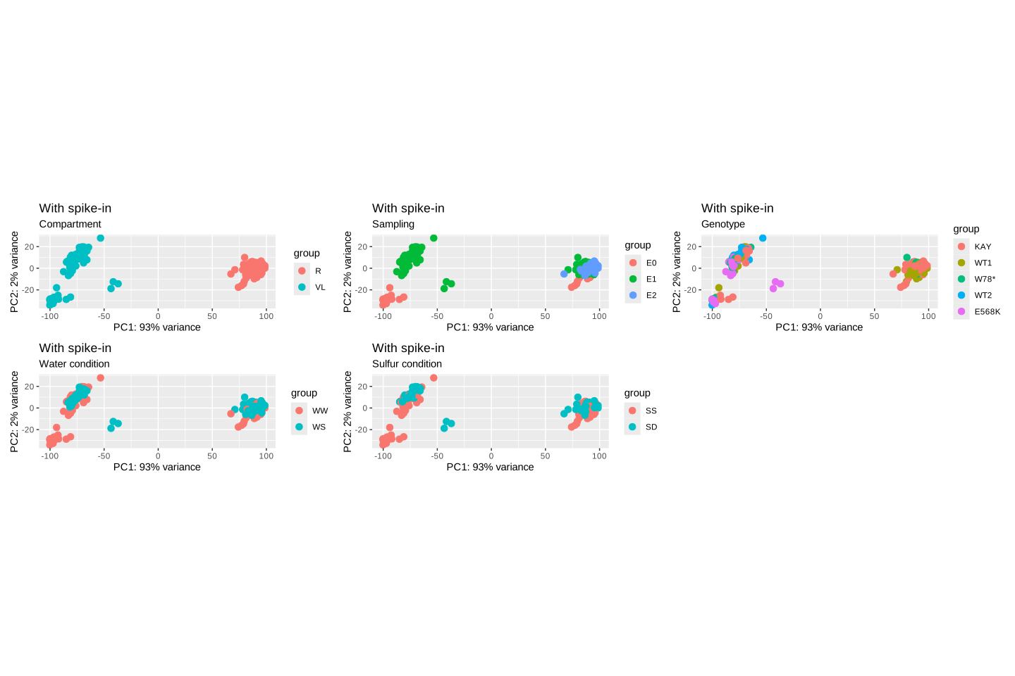{fig-align="center"} 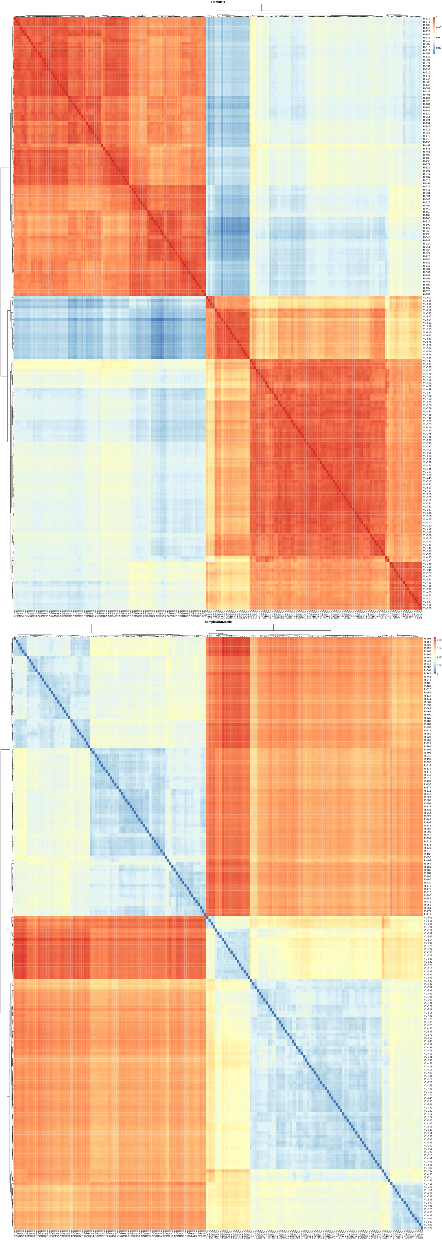{fig-align="center"} **I decided to analyze the data without using the exogenous spike-ins for normalization.** **So i remove the spike-ins genes (i.e begin by ERCC)**## Pre-filtering and normalize for full analyseWhile it is not necessary to pre-filter low count genes before running the DESeq2 functions, there are two reasons which make pre-filtering useful: by removing rows in which there are very few reads, we reduce the memory size of the dds data object, and we increase the speed of the transformation and testing functions within DESeq2. **Using vst() or varianceStabilizingTransformation() ?** This is a wrapper for the varianceStabilizingTransformation (VST) that provides much faster estimation of the dispersion trend used to determine the formula for the VST. The speed-up is accomplished by subsetting to a smaller number of genes in order to estimate this dispersion trend. The subset of genes is chosen deterministically, to span the range of genes' mean normalized count. This wrapper for the VST is not blind to the experimental design: the sample covariate information is used to estimate the global trend of genes' dispersion values over the genes' mean normalized count. It can be made strictly blind to experimental design by first assigning a design of \~1 before running this function, or by avoiding subsetting and using varianceStabilizingTransformation.This function calculates a variance stabilizing transformation (VST) from the fitted dispersion-mean relation(s) and then transforms the count data (normalized by division by the size factors or normalization factors), yielding a matrix of values which are now approximately homoskedastic (having constant variance along the range of mean values). The transformation also normalizes with respect to library size. The rlog is less sensitive to size factors, which can be an issue when size factors vary widely. These transformations are useful when checking for outliers or as input for machine learning techniques such as clustering or linear discriminant analysis.Change level to adapte deseq (control is WT and OT for (Well watered and Optimal sulfure condition) )full dataset to (root and vegetative leaves (VL)) to compare the influence of the stress depending of the type of sampling and genotype. **VL are more sensible to stress ?**. I can do that only at E1 and only for WT1 (Caméor) and KAY (Kayane). ```{r, eval=F}df_count <- read_csv(file = here::here("data/rnaseq/raw_counts.csv"), show_col_types = FALSE) %>% dplyr::rename(psat = 1) %>% column_to_rownames("psat")sample_list_rnaseq <- read_csv(file = here::here("data/rnaseq/output/sample_list_rnaseq.csv"),show_col_types = FALSE) %>% dplyr::mutate( genotype = forcats::fct_relevel(genotype, "KAY", "WT1", "W78*", "WT2", "E568K"), water_condition = forcats::fct_relevel(water_condition, "WW", "WS"), sulfur_condition = forcats::fct_relevel(sulfur_condition, "SS", "SD"), sampling = forcats::fct_relevel(sampling, "E0", "E1", "E2"), edaphic_condition = forcats::fct_relevel(edaphic_condition, "WW_SS", "WW_SD", "WS_SS", "WS_SD"), compartment = forcats::fct_relevel(compartment, "VL", "R"), condition = forcats::fct_relevel(condition, "KAY_WW_SS", "KAY_WW_SD", "KAY_WS_SS", "KAY_WS_SD", "WT1_WW_SS", "WT1_WW_SD", "WT1_WS_SS", "WT1_WS_SD", "W78*_WW_SS", "W78*_WW_SD", "W78*_WS_SS", "W78*_WS_SD", "WT2_WW_SS", "WT2_WW_SD", "WT2_WS_SS", "WT2_WS_SD", "E568K_WW_SS","E568K_WW_SD", "E568K_WS_SS", "E568K_WS_SD" ) )## 0. Make sure the *columns* of the count matrix are exactly## the samples you keep in your metadata ------------------sample_list_rnaseq_full <- sample_list_rnaseq### filtercount_table_full<-df_count %>% dplyr::select(sample_list_rnaseq_full$sample_id)# ## 1. Prefilter: keep genes with ≥10 counts in ≥90 % of samples ----------# keep <- rowSums(count_table_vl >= 10) >= 0.9 * ncol(count_table_vl)# count_table_vl_filt <- count_table_vl[keep, ]# ## 1. Prefilter: Keep a gene if it has ≥ 10 raw counts in at least min_samples libraries within any one experimental group.group <- with(sample_list_rnaseq_full, # metadata tibble interaction(compartment, sampling, genotype, water_condition, sulfur_condition, drop = TRUE)) # drop unused levels## 1B Apply the filtermin_count <- 10 # threshold on raw countsmin_samples <- 3 # ≥ this many libraries in the same groupkeep_manual <- apply(count_table_full, 1, function(cnts) { # cnts = vector of counts for ONE gene across all samples hits_per_group <- tapply(cnts >= min_count, group, sum) max(hits_per_group) >= min_samples})sum(keep_manual) # how many genes survive?count_table_filt <- count_table_full[keep_manual, ]## 2. Build DESeqDataSet and run DESeq -------------------------------### deseqdds_full <-DESeqDataSetFromMatrix(countData = count_table_filt, colData=sample_list_rnaseq_full, design = ~compartment+sampling+genotype+water_condition+sulfur_condition+genotype:water_condition+genotype:sulfur_condition+water_condition:sulfur_condition+genotype:water_condition:sulfur_condition)dds_full_1 <- DESeq(dds_full)# see https://www.biostars.org/p/9573278/ for spike-ins normalization# Change control conditiondds_full_1$water_condition = relevel(dds_full_1$water_condition, "WW")dds_full_1$sulfur_condition = relevel(dds_full_1$sulfur_condition, "SS")## 3. Transformations for visualisation -------------------------------rld_full <- rlog(dds_full_1, blind = TRUE)vst_full <- vst(dds_full_1, blind = TRUE)# all the info of the dds filter resultsNames(dds_full_1)colData(dds_full_1) # to know metadatadesign(dds_full_1)################## comparison VL to Root at E1 without stress condition ####################################################################### 0. Make sure the *columns* of the count matrix are exactly## the samples you keep in your metadata ------------------sample_list_rnaseq_comparison_compartment_E1_WW_SS <- sample_list_rnaseq %>% filter(sampling == "E1", genotype %in% c("WT1", "KAY"), edaphic_condition == "WW_SS" )### filtercount_table_comparison_compartment_E1_WW_SS<-df_count %>% dplyr::select(sample_list_rnaseq_comparison_compartment_E1_WW_SS$sample_id)# ## 1. Prefilter: keep genes with ≥10 counts in ≥90 % of samples ----------# keep <- rowSums(count_table_vl >= 10) >= 0.9 * ncol(count_table_vl)# count_table_vl_filt <- count_table_vl[keep, ]# ## 1. Prefilter: Keep a gene if it has ≥ 10 raw counts in at least min_samples libraries within any one experimental group.group <- with(sample_list_rnaseq_comparison_compartment_E1_WW_SS, # metadata tibble interaction(compartment, genotype, drop = TRUE)) # drop unused levels## 1B Apply the filtermin_count <- 10 # threshold on raw countsmin_samples <- 3 # ≥ this many libraries in the same groupkeep_manual <- apply(count_table_comparison_compartment_E1_WW_SS, 1, function(cnts) { # cnts = vector of counts for ONE gene across all samples hits_per_group <- tapply(cnts >= min_count, group, sum) max(hits_per_group) >= min_samples})sum(keep_manual) # how many genes survive?count_table_filt <- count_table_comparison_compartment_E1_WW_SS[keep_manual, ]## 2. Build DESeqDataSet and run DESeq -------------------------------### deseqdds_comparison_compartment_E1_WW_SS <-DESeqDataSetFromMatrix(countData = count_table_filt, colData=sample_list_rnaseq_comparison_compartment_E1_WW_SS, design = ~compartment+genotype+compartment:genotype)dds_comparison_compartment_E1_WW_SS_1 <- DESeq(dds_comparison_compartment_E1_WW_SS)# see https://www.biostars.org/p/9573278/ for spike-ins normalization## 3. Transformations for visualisation -------------------------------rld_comparison_compartment_E1_WW_SS <- rlog(dds_comparison_compartment_E1_WW_SS_1, blind = TRUE)vst_comparison_compartment_E1_WW_SS <- vst(dds_comparison_compartment_E1_WW_SS_1, blind = TRUE)# all the info of the dds filter resultsNames(dds_comparison_compartment_E1_WW_SS_1)colData(dds_comparison_compartment_E1_WW_SS_1) # to know metadatadesign(dds_comparison_compartment_E1_WW_SS_1)################## comparison VL to Root at E0 AND E1 without stress condition ####################################################################### 0. Make sure the *columns* of the count matrix are exactly## the samples you keep in your metadata ------------------sample_list_rnaseq_comparison_compartment_E0_E1_WW_SS <- sample_list_rnaseq %>% filter(sampling %in% c("E0","E1"), genotype %in% c("WT1", "KAY"), edaphic_condition == "WW_SS" )### filtercount_table_comparison_compartment_E0_E1_WW_SS<-df_count %>% dplyr::select(sample_list_rnaseq_comparison_compartment_E0_E1_WW_SS$sample_id)# ## 1. Prefilter: keep genes with ≥10 counts in ≥90 % of samples ----------# keep <- rowSums(count_table_vl >= 10) >= 0.9 * ncol(count_table_vl)# count_table_vl_filt <- count_table_vl[keep, ]# ## 1. Prefilter: Keep a gene if it has ≥ 10 raw counts in at least min_samples libraries within any one experimental group.group <- with(sample_list_rnaseq_comparison_compartment_E0_E1_WW_SS, # metadata tibble interaction(compartment, sampling, genotype, drop = TRUE)) # drop unused levels## 1B Apply the filtermin_count <- 10 # threshold on raw countsmin_samples <- 3 # ≥ this many libraries in the same groupkeep_manual <- apply(count_table_comparison_compartment_E0_E1_WW_SS, 1, function(cnts) { # cnts = vector of counts for ONE gene across all samples hits_per_group <- tapply(cnts >= min_count, group, sum) max(hits_per_group) >= min_samples})sum(keep_manual) # how many genes survive?count_table_filt <- count_table_comparison_compartment_E0_E1_WW_SS[keep_manual, ]## 2. Build DESeqDataSet and run DESeq -------------------------------### deseqdds_comparison_compartment_E0_E1_WW_SS <-DESeqDataSetFromMatrix(countData = count_table_filt, colData=sample_list_rnaseq_comparison_compartment_E0_E1_WW_SS, design = ~compartment+sampling+genotype+compartment:genotype+compartment:sampling+sampling:genotype)dds_comparison_compartment_E0_E1_WW_SS_1 <- DESeq(dds_comparison_compartment_E0_E1_WW_SS)# see https://www.biostars.org/p/9573278/ for spike-ins normalization## 3. Transformations for visualisation -------------------------------rld_comparison_compartment_E0_E1_WW_SS <- rlog(dds_comparison_compartment_E0_E1_WW_SS_1, blind = TRUE)vst_comparison_compartment_E0_E1_WW_SS <- vst(dds_comparison_compartment_E0_E1_WW_SS_1, blind = TRUE)# all the info of the dds filter resultsNames(dds_comparison_compartment_E0_E1_WW_SS_1)colData(dds_comparison_compartment_E0_E1_WW_SS_1) # to know metadatadesign(dds_comparison_compartment_E0_E1_WW_SS_1)################## comparison genotype for VL at E0, E1 and E2 (ony for vegetative leaves) without stress condition ####################################################################### 0. Make sure the *columns* of the count matrix are exactly## the samples you keep in your metadata ------------------sample_list_rnaseq_comparison_genotype_E0_E1_WW_SS_VL <- sample_list_rnaseq %>% filter(sampling %in% c("E0","E1"), genotype %in% c("WT1", "KAY"), edaphic_condition == "WW_SS", compartment == "VL" )### filtercount_table_comparison_genotype_E0_E1_WW_SS_VL<-df_count %>% dplyr::select(sample_list_rnaseq_comparison_genotype_E0_E1_WW_SS_VL$sample_id)# ## 1. Prefilter: Keep a gene if it has ≥ 10 raw counts in at least min_samples libraries within any one experimental group.group <- with(sample_list_rnaseq_comparison_genotype_E0_E1_WW_SS_VL, # metadata tibble interaction(sampling, genotype, drop = TRUE)) # drop unused levels## 1B Apply the filtermin_count <- 10 # threshold on raw countsmin_samples <- 3 # ≥ this many libraries in the same groupkeep_manual <- apply(count_table_comparison_genotype_E0_E1_WW_SS_VL, 1, function(cnts) { # cnts = vector of counts for ONE gene across all samples hits_per_group <- tapply(cnts >= min_count, group, sum) max(hits_per_group) >= min_samples})sum(keep_manual) # how many genes survive?count_table_filt <- count_table_comparison_genotype_E0_E1_WW_SS_VL[keep_manual, ]## 2. Build DESeqDataSet and run DESeq -------------------------------### deseqdds_comparison_genotype_E0_E1_WW_SS_VL <-DESeqDataSetFromMatrix(countData = count_table_filt, colData=sample_list_rnaseq_comparison_genotype_E0_E1_WW_SS_VL, design = ~sampling+genotype+sampling:genotype)dds_comparison_genotype_E0_E1_WW_SS_VL_1 <- DESeq(dds_comparison_genotype_E0_E1_WW_SS_VL)# see https://www.biostars.org/p/9573278/ for spike-ins normalization## 3. Transformations for visualisation -------------------------------rld_comparison_genotype_E0_E1_WW_SS_VL <- rlog(dds_comparison_genotype_E0_E1_WW_SS_VL_1, blind = TRUE)vst_comparison_genotype_E0_E1_WW_SS_VL <- vst(dds_comparison_genotype_E0_E1_WW_SS_VL_1, blind = TRUE)# all the info of the dds filter resultsNames(dds_comparison_genotype_E0_E1_WW_SS_VL_1)colData(dds_comparison_genotype_E0_E1_WW_SS_VL_1) # to know metadatadesign(dds_comparison_genotype_E0_E1_WW_SS_VL_1)################## comparison VL to Root at E0, E1 and E2 (ony for root) without stress condition ####################################################################### 0. Make sure the *columns* of the count matrix are exactly## the samples you keep in your metadata ------------------sample_list_rnaseq_comparison_compartment_E0_E1_E2_WW_SS_R <- sample_list_rnaseq %>% filter(sampling %in% c("E0","E1", "E2"), genotype %in% c("WT1", "KAY"), edaphic_condition == "WW_SS", compartment == "R" )### filtercount_table_comparison_compartment_E0_E1_E2_WW_SS_R<-df_count %>% dplyr::select(sample_list_rnaseq_comparison_compartment_E0_E1_E2_WW_SS_R$sample_id)# ## 1. Prefilter: keep genes with ≥10 counts in ≥90 % of samples ----------# keep <- rowSums(count_table_vl >= 10) >= 0.9 * ncol(count_table_vl)# count_table_vl_filt <- count_table_vl[keep, ]# ## 1. Prefilter: Keep a gene if it has ≥ 10 raw counts in at least min_samples libraries within any one experimental group.group <- with(sample_list_rnaseq_comparison_compartment_E0_E1_E2_WW_SS_R, # metadata tibble interaction(sampling, genotype, drop = TRUE)) # drop unused levels## 1B Apply the filtermin_count <- 10 # threshold on raw countsmin_samples <- 3 # ≥ this many libraries in the same groupkeep_manual <- apply(count_table_comparison_compartment_E0_E1_E2_WW_SS_R, 1, function(cnts) { # cnts = vector of counts for ONE gene across all samples hits_per_group <- tapply(cnts >= min_count, group, sum) max(hits_per_group) >= min_samples})sum(keep_manual) # how many genes survive?count_table_filt <- count_table_comparison_compartment_E0_E1_E2_WW_SS_R[keep_manual, ]## 2. Build DESeqDataSet and run DESeq -------------------------------### deseqdds_comparison_compartment_E0_E1_E2_WW_SS_R <-DESeqDataSetFromMatrix(countData = count_table_filt, colData=sample_list_rnaseq_comparison_compartment_E0_E1_E2_WW_SS_R, design = ~sampling+genotype+sampling:genotype)dds_comparison_compartment_E0_E1_E2_WW_SS_R_1 <- DESeq(dds_comparison_compartment_E0_E1_E2_WW_SS_R)# see https://www.biostars.org/p/9573278/ for spike-ins normalization## 3. Transformations for visualisation -------------------------------rld_comparison_compartment_E0_E1_E2_WW_SS_R <- rlog(dds_comparison_compartment_E0_E1_E2_WW_SS_R_1, blind = TRUE)vst_comparison_compartment_E0_E1_E2_WW_SS_R <- vst(dds_comparison_compartment_E0_E1_E2_WW_SS_R_1, blind = TRUE)# all the info of the dds filter resultsNames(dds_comparison_compartment_E0_E1_E2_WW_SS_R_1)colData(dds_comparison_compartment_E0_E1_E2_WW_SS_R_1) # to know metadatadesign(dds_comparison_compartment_E0_E1_E2_WW_SS_R_1)################## comparison VL to Root at E1 ####################################################################### 0. Make sure the *columns* of the count matrix are exactly## the samples you keep in your metadata ------------------sample_list_rnaseq_comparison_compartment <- sample_list_rnaseq %>% filter(sampling == "E1", genotype %in% c("WT1", "KAY"))### filtercount_table_comparison_compartment<-df_count %>% dplyr::select(sample_list_rnaseq_comparison_compartment$sample_id)# ## 1. Prefilter: keep genes with ≥10 counts in ≥90 % of samples ----------# keep <- rowSums(count_table_vl >= 10) >= 0.9 * ncol(count_table_vl)# count_table_vl_filt <- count_table_vl[keep, ]# ## 1. Prefilter: Keep a gene if it has ≥ 10 raw counts in at least min_samples libraries within any one experimental group.group <- with(sample_list_rnaseq_comparison_compartment, # metadata tibble interaction(compartment, genotype, water_condition, sulfur_condition, drop = TRUE)) # drop unused levels## 1B Apply the filtermin_count <- 10 # threshold on raw countsmin_samples <- 3 # ≥ this many libraries in the same groupkeep_manual <- apply(count_table_comparison_compartment, 1, function(cnts) { # cnts = vector of counts for ONE gene across all samples hits_per_group <- tapply(cnts >= min_count, group, sum) max(hits_per_group) >= min_samples})sum(keep_manual) # how many genes survive?count_table_filt <- count_table_comparison_compartment[keep_manual, ]## 2. Build DESeqDataSet and run DESeq -------------------------------### deseqdds_comparison_compartment <-DESeqDataSetFromMatrix(countData = count_table_filt, colData=sample_list_rnaseq_comparison_compartment, design = ~compartment+genotype+water_condition+sulfur_condition+genotype:water_condition+genotype:sulfur_condition+water_condition:sulfur_condition+genotype:water_condition:sulfur_condition)dds_comparison_compartment_1 <- DESeq(dds_comparison_compartment)# see https://www.biostars.org/p/9573278/ for spike-ins normalization## 3. Transformations for visualisation -------------------------------rld_comparison_compartment <- rlog(dds_comparison_compartment_1, blind = TRUE)vst_comparison_compartment <- vst(dds_comparison_compartment_1, blind = TRUE)# all the info of the dds filter resultsNames(dds_comparison_compartment_1)colData(dds_comparison_compartment_1) # to know metadatadesign(dds_comparison_compartment_1)################## comparison VL to Root at E0 ####################################################################### 0. Make sure the *columns* of the count matrix are exactly## the samples you keep in your metadata ------------------sample_list_rnaseq_comparison_compartment_E0 <- sample_list_rnaseq %>% filter(sampling == "E0", genotype %in% c("WT1", "KAY"))### filtercount_table_comparison_compartment_E0<-df_count %>% dplyr::select(sample_list_rnaseq_comparison_compartment_E0$sample_id)# ## 1. Prefilter: keep genes with ≥10 counts in ≥90 % of samples ----------# keep <- rowSums(count_table_vl >= 10) >= 0.9 * ncol(count_table_vl)# count_table_vl_filt <- count_table_vl[keep, ]# ## 1. Prefilter: Keep a gene if it has ≥ 10 raw counts in at least min_samples libraries within any one experimental group.group <- with(sample_list_rnaseq_comparison_compartment_E0, # metadata tibble interaction(compartment, genotype, drop = TRUE)) # drop unused levels## 1B Apply the filtermin_count <- 10 # threshold on raw countsmin_samples <- 3 # ≥ this many libraries in the same groupkeep_manual <- apply(count_table_comparison_compartment_E0, 1, function(cnts) { # cnts = vector of counts for ONE gene across all samples hits_per_group <- tapply(cnts >= min_count, group, sum) max(hits_per_group) >= min_samples})sum(keep_manual) # how many genes survive?count_table_filt <- count_table_comparison_compartment_E0[keep_manual, ]## 2. Build DESeqDataSet and run DESeq -------------------------------### deseqdds_comparison_compartment_E0 <-DESeqDataSetFromMatrix(countData = count_table_filt, colData=sample_list_rnaseq_comparison_compartment_E0, design = ~compartment+genotype+compartment:genotype)dds_comparison_compartment_E0_1 <- DESeq(dds_comparison_compartment_E0)# see https://www.biostars.org/p/9573278/ for spike-ins normalization## 3. Transformations for visualisation -------------------------------rld_comparison_compartment_E0 <- rlog(dds_comparison_compartment_E0_1, blind = TRUE)vst_comparison_compartment_E0 <- vst(dds_comparison_compartment_E0_1, blind = TRUE)# all the info of the dds filter resultsNames(dds_comparison_compartment_E0_1)colData(dds_comparison_compartment_E0_1) # to know metadatadesign(dds_comparison_compartment_E0_1)################## comparison Root KAY and WT1 at E2 ####################################################################### 0. Make sure the *columns* of the count matrix are exactly## the samples you keep in your metadata ------------------sample_list_rnaseq_comparison_root_genotype_E2_WW_SS <- sample_list_rnaseq %>% filter(sampling == "E2", genotype %in% c("WT1", "KAY"), edaphic_condition == "WW_SS")### filtercount_table_comparison_root_genotype_E2_WW_SS<-df_count %>% dplyr::select(sample_list_rnaseq_comparison_root_genotype_E2_WW_SS$sample_id)# ## 1. Prefilter: Keep a gene if it has ≥ 10 raw counts in at least min_samples libraries within any one experimental group.group <- with(sample_list_rnaseq_comparison_root_genotype_E2_WW_SS, # metadata tibble interaction(genotype, drop = TRUE)) # drop unused levels## 1B Apply the filtermin_count <- 10 # threshold on raw countsmin_samples <- 3 # ≥ this many libraries in the same groupkeep_manual <- apply(count_table_comparison_root_genotype_E2_WW_SS, 1, function(cnts) { # cnts = vector of counts for ONE gene across all samples hits_per_group <- tapply(cnts >= min_count, group, sum) max(hits_per_group) >= min_samples})sum(keep_manual) # how many genes survive?count_table_filt <- count_table_comparison_root_genotype_E2_WW_SS[keep_manual, ]## 2. Build DESeqDataSet and run DESeq -------------------------------### deseqdds_comparison_root_genotype_E2_WW_SS <-DESeqDataSetFromMatrix(countData = count_table_filt, colData=sample_list_rnaseq_comparison_root_genotype_E2_WW_SS, design = ~genotype)dds_comparison_root_genotype_E2_WW_SS_1 <- DESeq(dds_comparison_root_genotype_E2_WW_SS)# see https://www.biostars.org/p/9573278/ for spike-ins normalization## 3. Transformations for visualisation -------------------------------rld_comparison_root_genotype_E2_WW_SS <- rlog(dds_comparison_root_genotype_E2_WW_SS_1, blind = TRUE)vst_comparison_root_genotype_E2_WW_SS <- vst(dds_comparison_root_genotype_E2_WW_SS_1, blind = TRUE)# all the info of the dds filter resultsNames(dds_comparison_root_genotype_E2_WW_SS_1)colData(dds_comparison_root_genotype_E2_WW_SS_1) # to know metadatadesign(dds_comparison_root_genotype_E2_WW_SS_1)######################################################################################## export all importante valuesave(sample_list_rnaseq_full, dds_full, dds_full_1, rld_full, vst_full, file = here::here("data/rnaseq/output/full.RData"))save(sample_list_rnaseq_comparison_compartment, dds_comparison_compartment, dds_comparison_compartment_1, rld_comparison_compartment, vst_comparison_compartment, file = here::here("data/rnaseq/output/comparison_compartment.RData"))save(sample_list_rnaseq_comparison_compartment_E0, dds_comparison_compartment_E0, dds_comparison_compartment_E0_1, rld_comparison_compartment_E0, vst_comparison_compartment_E0, file = here::here("data/rnaseq/output/comparison_compartment_E0.RData"))save(sample_list_rnaseq_comparison_compartment_E1_WW_SS, dds_comparison_compartment_E1_WW_SS, dds_comparison_compartment_E1_WW_SS_1, rld_comparison_compartment_E1_WW_SS, vst_comparison_compartment_E1_WW_SS, file = here::here("data/rnaseq/output/comparison_compartment_E1_WW_SS.RData"))save(sample_list_rnaseq_comparison_compartment_E0_E1_WW_SS, dds_comparison_compartment_E0_E1_WW_SS, dds_comparison_compartment_E0_E1_WW_SS_1, rld_comparison_compartment_E0_E1_WW_SS, vst_comparison_compartment_E0_E1_WW_SS, file = here::here("data/rnaseq/output/comparison_compartment_E0_E1_WW_SS.RData"))save(sample_list_rnaseq_comparison_compartment_E0_E1_E2_WW_SS_R, dds_comparison_compartment_E0_E1_E2_WW_SS_R, dds_comparison_compartment_E0_E1_E2_WW_SS_R_1, rld_comparison_compartment_E0_E1_E2_WW_SS_R, vst_comparison_compartment_E0_E1_E2_WW_SS_R, file = here::here("data/rnaseq/output/comparison_compartment_E0_E1_E2_WW_SS_R.RData"))save(sample_list_rnaseq_comparison_genotype_E0_E1_WW_SS_VL, dds_comparison_genotype_E0_E1_WW_SS_VL, dds_comparison_genotype_E0_E1_WW_SS_VL_1, rld_comparison_genotype_E0_E1_WW_SS_VL, vst_comparison_genotype_E0_E1_WW_SS_VL, file = here::here("data/rnaseq/output/comparison_genotype_E0_E1_WW_SS_VL.RData"))save(sample_list_rnaseq_comparison_root_genotype_E2_WW_SS, dds_comparison_root_genotype_E2_WW_SS, dds_comparison_root_genotype_E2_WW_SS_1, rld_comparison_root_genotype_E2_WW_SS, vst_comparison_root_genotype_E2_WW_SS, file = here::here("data/rnaseq/output/comparison_root_genotype_E2_WW_SS.RData"))```**Subdivision of datasets for different scientific questions** Then filtration on the low count and normalization ```{r, eval=F}#data importationdf_count <- read_csv(file = here::here("data/rnaseq/raw_counts.csv"), show_col_types = FALSE) %>% dplyr::rename(psat = 1) %>% column_to_rownames("psat")sample_list_rnaseq <- read_csv(file = here::here("data/rnaseq/output/sample_list_rnaseq.csv"),show_col_types = FALSE) %>% dplyr::mutate( genotype = forcats::fct_relevel(genotype, "KAY", "WT1", "W78*", "WT2", "E568K"), water_condition = forcats::fct_relevel(water_condition, "WW", "WS"), sulfur_condition = forcats::fct_relevel(sulfur_condition, "SS", "SD"), sampling = forcats::fct_relevel(sampling, "E0", "E1", "E2"), edaphic_condition = forcats::fct_relevel(edaphic_condition, "WW_SS", "WW_SD", "WS_SS", "WS_SD"), compartment = forcats::fct_relevel(compartment, "VL", "R"), condition = forcats::fct_relevel(condition, "KAY_WW_SS", "KAY_WW_SD", "KAY_WS_SS", "KAY_WS_SD", "WT1_WW_SS", "WT1_WW_SD", "WT1_WS_SS", "WT1_WS_SD", "W78*_WW_SS", "W78*_WW_SD", "W78*_WS_SS", "W78*_WS_SD", "WT2_WW_SS", "WT2_WW_SD", "WT2_WS_SS", "WT2_WS_SD", "E568K_WW_SS","E568K_WW_SD", "E568K_WS_SS", "E568K_WS_SD" ) )#idem but for each group (compartement and sampling). first filter, filter lowcount, then normalize## For vegetative leaves ################################################################# 0. Make sure the *columns* of the count matrix are exactly## the samples you keep in your metadata ------------------sample_list_rnaseq_vl <- sample_list_rnaseq %>% filter(compartment == "VL")### filtercount_table_vl<-df_count %>% dplyr::select(sample_list_rnaseq_vl$sample_id)# ## 1. Prefilter: keep genes with ≥10 counts in ≥90 % of samples ----------# keep <- rowSums(count_table_vl >= 10) >= 0.9 * ncol(count_table_vl)# count_table_vl_filt <- count_table_vl[keep, ]# ## 1. Prefilter: Keep a gene if it has ≥ 10 raw counts in at least min_samples libraries within any one experimental group.group <- with(sample_list_rnaseq_vl, # metadata tibble interaction(sampling, genotype, water_condition, sulfur_condition, drop = TRUE)) # drop unused levels## 1B Apply the filtermin_count <- 10 # threshold on raw countsmin_samples <- 3 # ≥ this many libraries in the same groupkeep_manual <- apply(count_table_vl, 1, function(cnts) { # cnts = vector of counts for ONE gene across all samples hits_per_group <- tapply(cnts >= min_count, group, sum) max(hits_per_group) >= min_samples})sum(keep_manual) # how many genes survive?count_table_filt <- count_table_vl[keep_manual, ]## 2. Build DESeqDataSet and run DESeq -------------------------------### deseqdds_vl <-DESeqDataSetFromMatrix(countData = count_table_filt, colData=sample_list_rnaseq_vl, design = ~sampling+genotype+water_condition+sulfur_condition+genotype:water_condition+genotype:sulfur_condition+water_condition:sulfur_condition+genotype:water_condition:sulfur_condition)dds_vl_1 <- DESeq(dds_vl)# see https://www.biostars.org/p/9573278/ for spike-ins normalization## 3. Transformations for visualisation -------------------------------rld_vl <- rlog(dds_vl_1, blind = TRUE)vst_vl <- vst(dds_vl_1, blind = TRUE)# all the info of the dds filter resultsNames(dds_vl_1)colData(dds_vl_1) # to know metadatadesign(dds_vl_1)####################################################################################################################################### effet of the mutation for VL and if still there acording to the samplingsample_list_rnaseq_vl_WW_SS <- sample_list_rnaseq %>% filter(compartment == "VL", edaphic_condition == "WW_SS")### filtercount_table_vl_WW_SS<-df_count %>% dplyr::select(sample_list_rnaseq_vl_WW_SS$sample_id)# ## 1. Prefilter: keep genes with ≥10 counts in ≥90 % of samples ----------# keep <- rowSums(count_table_vl >= 10) >= 0.9 * ncol(count_table_vl)# count_table_vl_filt <- count_table_vl[keep, ]# ## 1. Prefilter: Keep a gene if it has ≥ 10 raw counts in at least min_samples libraries within any one experimental group.group <- with(sample_list_rnaseq_vl_WW_SS, # metadata tibble interaction(sampling, genotype, drop = TRUE)) # drop unused levels## 1B Apply the filtermin_count <- 10 # threshold on raw countsmin_samples <- 3 # ≥ this many libraries in the same groupkeep_manual <- apply(count_table_vl_WW_SS, 1, function(cnts) { # cnts = vector of counts for ONE gene across all samples hits_per_group <- tapply(cnts >= min_count, group, sum) max(hits_per_group) >= min_samples})sum(keep_manual) # how many genes survive?count_table_filt <- count_table_vl_WW_SS[keep_manual, ]## 2. Build DESeqDataSet and run DESeq -------------------------------### deseqdds_vl_WW_SS <-DESeqDataSetFromMatrix(countData = count_table_filt, colData=sample_list_rnaseq_vl_WW_SS, design = ~sampling+genotype+genotype:sampling)dds_vl_WW_SS_1 <- DESeq(dds_vl_WW_SS)# see https://www.biostars.org/p/9573278/ for spike-ins normalization## 3. Transformations for visualisation -------------------------------rld_vl_WW_SS <- rlog(dds_vl_WW_SS_1, blind = TRUE)vst_vl_WW_SS <- vst(dds_vl_WW_SS_1, blind = TRUE)# all the info of the dds filter resultsNames(dds_vl_WW_SS_1)colData(dds_vl_WW_SS_1) # to know metadatadesign(dds_vl_WW_SS_1)############################################################################################################################################# effet of the mutation for VL depending of the stress ?sample_list_rnaseq_vl_E1 <-sample_list_rnaseq %>% filter(compartment == "VL", sampling == "E1")### filtercount_table_vl_E1<-df_count %>% dplyr::select(sample_list_rnaseq_vl_E1$sample_id)group <- with(sample_list_rnaseq_vl_E1, # metadata tibble interaction(genotype, water_condition, sulfur_condition, drop = TRUE)) # drop unused levels## 1B Apply the filtermin_count <- 10 # threshold on raw countsmin_samples <- 3 # ≥ this many libraries in the same groupkeep_manual <- apply(count_table_vl_E1, 1, function(cnts) { # cnts = vector of counts for ONE gene across all samples hits_per_group <- tapply(cnts >= min_count, group, sum) max(hits_per_group) >= min_samples})sum(keep_manual) # how many genes survive?count_table_filt <- count_table_vl_E1[keep_manual, ]## 2. Build DESeqDataSet and run DESeq -------------------------------### deseqdds_vl_E1 <-DESeqDataSetFromMatrix(countData = count_table_filt, colData=sample_list_rnaseq_vl_E1, design = ~genotype+water_condition+sulfur_condition+genotype:water_condition+genotype:sulfur_condition+water_condition:sulfur_condition+genotype:water_condition:sulfur_condition)dds_vl_E1_1 <- DESeq(dds_vl_E1)# see https://www.biostars.org/p/9573278/ for spike-ins normalization## 3. Transformations for visualisation -------------------------------rld_vl_E1 <- rlog(dds_vl_E1_1, blind = TRUE)vst_vl_E1 <- vst(dds_vl_E1_1, blind = TRUE)# all the info of the dds filter resultsNames(dds_vl_E1_1)colData(dds_vl_E1_1) # to know metadatadesign(dds_vl_E1_1)############################################################################################################################################# effet of the mutation for VL depending of the stress but without interaction ?sample_list_rnaseq_vl_E1_condition <-sample_list_rnaseq %>% filter(compartment == "VL", sampling == "E1")### filtercount_table_vl_E1_condition<-df_count %>% dplyr::select(sample_list_rnaseq_vl_E1_condition$sample_id)group <- with(sample_list_rnaseq_vl_E1_condition, # metadata tibble interaction(condition, drop = TRUE)) # drop unused levels## 1B Apply the filtermin_count <- 10 # threshold on raw countsmin_samples <- 3 # ≥ this many libraries in the same groupkeep_manual <- apply(count_table_vl_E1_condition, 1, function(cnts) { # cnts = vector of counts for ONE gene across all samples hits_per_group <- tapply(cnts >= min_count, group, sum) max(hits_per_group) >= min_samples})sum(keep_manual) # how many genes survive?count_table_filt <- count_table_vl_E1_condition[keep_manual, ]## 2. Build DESeqDataSet and run DESeq -------------------------------### deseqdds_vl_E1_condition <-DESeqDataSetFromMatrix(countData = count_table_filt, colData=sample_list_rnaseq_vl_E1_condition, design = ~condition)dds_vl_E1_condition_1 <- DESeq(dds_vl_E1_condition)# see https://www.biostars.org/p/9573278/ for spike-ins normalization## 3. Transformations for visualisation -------------------------------rld_vl_E1_condition <- rlog(dds_vl_E1_condition_1, blind = TRUE)vst_vl_E1_condition <- vst(dds_vl_E1_condition_1, blind = TRUE)# all the info of the dds filter resultsNames(dds_vl_E1_condition_1)colData(dds_vl_E1_condition_1) # to know metadatadesign(dds_vl_E1_condition_1)############################################################################################################################################# for root #####################################################################sample_list_rnaseq_root <- sample_list_rnaseq %>% filter(compartment == "R")### filtercount_table_root<-df_count %>% dplyr::select(sample_list_rnaseq_root$sample_id)group <- with(sample_list_rnaseq_root, # metadata tibble interaction(sampling, genotype, water_condition, sulfur_condition, drop = TRUE)) ## 1B Apply the filtermin_count <- 10 # threshold on raw countsmin_samples <- 3 # ≥ this many libraries in the same groupkeep_manual <- apply(count_table_root, 1, function(cnts) { # cnts = vector of counts for ONE gene across all samples hits_per_group <- tapply(cnts >= min_count, group, sum) max(hits_per_group) >= min_samples})sum(keep_manual) # how many genes survive?count_table_filt <- count_table_root[keep_manual, ]## 2. Build DESeqDataSet and run DESeq -------------------------------### deseqdds_root <-DESeqDataSetFromMatrix(countData = count_table_filt, colData=sample_list_rnaseq_root, design = ~sampling+genotype+water_condition+sulfur_condition+genotype:water_condition+genotype:sulfur_condition+water_condition:sulfur_condition+genotype:water_condition:sulfur_condition)dds_root_1 <- DESeq(dds_root)# see https://www.biostars.org/p/9573278/ for spike-ins normalization## 3. Transformations for visualisation -------------------------------rld_root <- rlog(dds_root_1, blind = TRUE)vst_root <- vst(dds_root_1, blind = TRUE)# all the info of the dds filter resultsNames(dds_root_1)colData(dds_root_1) # to know metadatadesign(dds_root_1)############################################################################################################################################# effet of the sampling and stress condition on kayane and WT Cameor for root. What is the difference between the two genotype ? sample_list_rnaseq_root_sampling <-sample_list_rnaseq %>% filter(compartment == "R", genotype %in% c("KAY", "WT1"))### filtercount_table_root_sampling<-df_count %>% dplyr::select(sample_list_rnaseq_root_sampling$sample_id)group <- with(sample_list_rnaseq_root_sampling, # metadata tibble interaction(sampling, genotype, water_condition, sulfur_condition, drop = TRUE)) ## 1B Apply the filtermin_count <- 10 # threshold on raw countsmin_samples <- 3 # ≥ this many libraries in the same groupkeep_manual <- apply(count_table_root_sampling, 1, function(cnts) { # cnts = vector of counts for ONE gene across all samples hits_per_group <- tapply(cnts >= min_count, group, sum) max(hits_per_group) >= min_samples})sum(keep_manual) # how many genes survive?count_table_filt <- count_table_root_sampling[keep_manual, ]## 2. Build DESeqDataSet and run DESeq -------------------------------### deseqdds_root_sampling <-DESeqDataSetFromMatrix(countData = count_table_filt, colData=sample_list_rnaseq_root_sampling, design = ~sampling+genotype+water_condition+sulfur_condition+genotype:water_condition+genotype:sulfur_condition+water_condition:sulfur_condition+genotype:water_condition:sulfur_condition)dds_root_sampling_1 <- DESeq(dds_root_sampling)# see https://www.biostars.org/p/9573278/ for spike-ins normalization## 3. Transformations for visualisation -------------------------------rld_root_sampling <- rlog(dds_root_sampling_1, blind = TRUE)vst_root_sampling <- vst(dds_root_sampling_1, blind = TRUE)# all the info of the dds filter resultsNames(dds_root_sampling_1)colData(dds_root_sampling_1) # to know metadatadesign(dds_root_sampling_1)############################################################################################################################################# effet of the stress on root and effect of the mutationsample_list_rnaseq_root_E1_WT_Mut <- sample_list_rnaseq %>% filter(compartment == "R", sampling == "E1", genotype %in% c("WT1", "W78*"))### filtercount_table_root_E1_WT_Mut<-df_count %>% dplyr::select(sample_list_rnaseq_root_E1_WT_Mut$sample_id)group <- with(sample_list_rnaseq_root_E1_WT_Mut, # metadata tibble interaction(genotype, water_condition, sulfur_condition, drop = TRUE)) ## 1B Apply the filtermin_count <- 10 # threshold on raw countsmin_samples <- 3 # ≥ this many libraries in the same groupkeep_manual <- apply(count_table_root_E1_WT_Mut, 1, function(cnts) { # cnts = vector of counts for ONE gene across all samples hits_per_group <- tapply(cnts >= min_count, group, sum) max(hits_per_group) >= min_samples})sum(keep_manual) # how many genes survive?count_table_filt <- count_table_root_E1_WT_Mut[keep_manual, ]## 2. Build DESeqDataSet and run DESeq -------------------------------### deseqdds_root_E1_WT_Mut <-DESeqDataSetFromMatrix(countData = count_table_filt, colData=sample_list_rnaseq_root_E1_WT_Mut, design = ~genotype+water_condition+sulfur_condition+genotype:water_condition+genotype:sulfur_condition+water_condition:sulfur_condition+genotype:water_condition:sulfur_condition)dds_root_E1_WT_Mut_1 <- DESeq(dds_root_E1_WT_Mut)# see https://www.biostars.org/p/9573278/ for spike-ins normalization## 3. Transformations for visualisation -------------------------------rld_root_E1_WT_Mut <- rlog(dds_root_E1_WT_Mut_1, blind = TRUE)vst_root_E1_WT_Mut <- vst(dds_root_E1_WT_Mut_1, blind = TRUE)# all the info of the dds filter resultsNames(dds_root_E1_WT_Mut_1)colData(dds_root_E1_WT_Mut_1) # to know metadatadesign(dds_root_E1_WT_Mut_1)############################################################################################################################################# effet of the stress on root at E1 on each genotypesample_list_rnaseq_R_E1 <- sample_list_rnaseq %>% filter(compartment == "R", sampling == "E1" )### filtercount_table_R_E1<-df_count %>% dplyr::select(sample_list_rnaseq_R_E1$sample_id)group <- with(sample_list_rnaseq_R_E1, # metadata tibble interaction(genotype, water_condition, sulfur_condition, drop = TRUE)) ## 1B Apply the filtermin_count <- 10 # threshold on raw countsmin_samples <- 3 # ≥ this many libraries in the same groupkeep_manual <- apply(count_table_R_E1, 1, function(cnts) { # cnts = vector of counts for ONE gene across all samples hits_per_group <- tapply(cnts >= min_count, group, sum) max(hits_per_group) >= min_samples})sum(keep_manual) # how many genes survive?count_table_filt <- count_table_R_E1[keep_manual, ]## 2. Build DESeqDataSet and run DESeq -------------------------------### deseqdds_R_E1 <-DESeqDataSetFromMatrix(countData = count_table_filt, colData=sample_list_rnaseq_R_E1, design = ~genotype+water_condition+sulfur_condition+genotype:water_condition+genotype:sulfur_condition+water_condition:sulfur_condition+genotype:water_condition:sulfur_condition)dds_R_E1_1 <- DESeq(dds_R_E1)# see https://www.biostars.org/p/9573278/ for spike-ins normalization## 3. Transformations for visualisation -------------------------------rld_R_E1 <- rlog(dds_R_E1_1, blind = TRUE)vst_R_E1 <- vst(dds_R_E1_1, blind = TRUE)# all the info of the dds filter resultsNames(dds_R_E1_1)colData(dds_R_E1_1) # to know metadatadesign(dds_R_E1_1)############################################################################################################################################# effet of the mutation for R depending of the stress but without interaction ?sample_list_rnaseq_R_E1_condition <-sample_list_rnaseq %>% filter(compartment == "R", sampling == "E1")### filtercount_table_R_E1_condition<-df_count %>% dplyr::select(sample_list_rnaseq_R_E1_condition$sample_id)group <- with(sample_list_rnaseq_R_E1_condition, # metadata tibble interaction(condition, drop = TRUE)) # drop unused levels## 1B Apply the filtermin_count <- 10 # threshold on raw countsmin_samples <- 3 # ≥ this many libraries in the same groupkeep_manual <- apply(count_table_R_E1_condition, 1, function(cnts) { # cnts = vector of counts for ONE gene across all samples hits_per_group <- tapply(cnts >= min_count, group, sum) max(hits_per_group) >= min_samples})sum(keep_manual) # how many genes survive?count_table_filt <- count_table_R_E1_condition[keep_manual, ]## 2. Build DESeqDataSet and run DESeq -------------------------------### deseqdds_R_E1_condition <-DESeqDataSetFromMatrix(countData = count_table_filt, colData=sample_list_rnaseq_R_E1_condition, design = ~condition)dds_R_E1_condition_1 <- DESeq(dds_R_E1_condition)# see https://www.biostars.org/p/9573278/ for spike-ins normalization## 3. Transformations for visualisation -------------------------------rld_R_E1_condition <- rlog(dds_R_E1_condition_1, blind = TRUE)vst_R_E1_condition <- vst(dds_R_E1_condition_1, blind = TRUE)# all the info of the dds filter resultsNames(dds_R_E1_condition_1)colData(dds_R_E1_condition_1) # to know metadatadesign(dds_R_E1_condition_1)#######################################################################################################################################sample_list_rnaseq_R_KAY_WT1_E0_E1_E2 <-sample_list_rnaseq %>% filter(compartment == "R", genotype %in% c("KAY", "WT1"))### filtercount_table_R_KAY_WT1_E0_E1_E2<-df_count %>% dplyr::select(sample_list_rnaseq_R_KAY_WT1_E0_E1_E2$sample_id)group <- with(sample_list_rnaseq_R_KAY_WT1_E0_E1_E2, # metadata tibble interaction(sampling, genotype, water_condition, sulfur_condition, drop = TRUE)) # drop unused levels## 1B Apply the filtermin_count <- 10 # threshold on raw countsmin_samples <- 3 # ≥ this many libraries in the same groupkeep_manual <- apply(count_table_R_KAY_WT1_E0_E1_E2, 1, function(cnts) { # cnts = vector of counts for ONE gene across all samples hits_per_group <- tapply(cnts >= min_count, group, sum) max(hits_per_group) >= min_samples})sum(keep_manual) # how many genes survive?count_table_filt <- count_table_R_KAY_WT1_E0_E1_E2[keep_manual, ]## 2. Build DESeqDataSet and run DESeq -------------------------------### deseqdds_R_KAY_WT1_E0_E1_E2 <-DESeqDataSetFromMatrix(countData = count_table_filt, colData=sample_list_rnaseq_R_KAY_WT1_E0_E1_E2, design = ~sampling+edaphic_condition+genotype)dds_R_KAY_WT1_E0_E1_E2_1 <- DESeq(dds_R_KAY_WT1_E0_E1_E2)# see https://www.biostars.org/p/9573278/ for spike-ins normalization## 3. Transformations for visualisation -------------------------------rld_R_KAY_WT1_E0_E1_E2 <- rlog(dds_R_KAY_WT1_E0_E1_E2_1, blind = TRUE)vst_R_KAY_WT1_E0_E1_E2 <- vst(dds_R_KAY_WT1_E0_E1_E2_1, blind = TRUE)# all the info of the dds filter resultsNames(dds_R_KAY_WT1_E0_E1_E2_1)colData(dds_R_KAY_WT1_E0_E1_E2_1) # to know metadatadesign(dds_R_KAY_WT1_E0_E1_E2_1)######################################################################################################################################## find the recovery genees and stress specifique genes for Rsample_list_rnaseq_R_KAY_WT1_E1_E2 <-sample_list_rnaseq %>% filter(compartment == "R", genotype %in% c("KAY", "WT1"), sampling %in% c("E1", "E2"))### filtercount_table_R_KAY_WT1_E1_E2<-df_count %>% dplyr::select(sample_list_rnaseq_R_KAY_WT1_E1_E2$sample_id)group <- with(sample_list_rnaseq_R_KAY_WT1_E1_E2, # metadata tibble interaction(sampling, #genotype, # not take in count the genotype water_condition, sulfur_condition, drop = TRUE)) # drop unused levels## 1B Apply the filtermin_count <- 10 # threshold on raw countsmin_samples <- 3 # ≥ this many libraries in the same groupkeep_manual <- apply(count_table_R_KAY_WT1_E1_E2, 1, function(cnts) { # cnts = vector of counts for ONE gene across all samples hits_per_group <- tapply(cnts >= min_count, group, sum) max(hits_per_group) >= min_samples})sum(keep_manual) # how many genes survive?count_table_filt <- count_table_R_KAY_WT1_E1_E2[keep_manual, ]## 2. Build DESeqDataSet and run DESeq -------------------------------### deseqdds_R_KAY_WT1_E1_E2 <-DESeqDataSetFromMatrix(countData = count_table_filt, colData=sample_list_rnaseq_R_KAY_WT1_E1_E2, design = ~sampling*edaphic_condition)dds_R_KAY_WT1_E1_E2_1 <- DESeq(dds_R_KAY_WT1_E1_E2)# see https://www.biostars.org/p/9573278/ for spike-ins normalization## 3. Transformations for visualisation -------------------------------rld_R_KAY_WT1_E1_E2 <- rlog(dds_R_KAY_WT1_E1_E2_1, blind = TRUE)vst_R_KAY_WT1_E1_E2 <- vst(dds_R_KAY_WT1_E1_E2_1, blind = TRUE)# all the info of the dds filter resultsNames(dds_R_KAY_WT1_E1_E2_1)colData(dds_R_KAY_WT1_E1_E2_1) # to know metadatadesign(dds_R_KAY_WT1_E1_E2_1)######################################################################################################################################## find the recovery genees and stress specifique genes for R (without interaction)sample_list_rnaseq_R_KAY_WT1_E1_E2_condition <-sample_list_rnaseq %>% filter(compartment == "R", genotype %in% c("KAY", "WT1"), sampling %in% c("E1", "E2")) %>% mutate(sampling_condition = paste0(sampling, "_", condition))### filtercount_table_R_KAY_WT1_E1_E2_condition<-df_count %>% dplyr::select(sample_list_rnaseq_R_KAY_WT1_E1_E2_condition$sample_id)group <- with(sample_list_rnaseq_R_KAY_WT1_E1_E2_condition, # metadata tibble interaction(sampling_condition, drop = TRUE)) # drop unused levels## 1B Apply the filtermin_count <- 10 # threshold on raw countsmin_samples <- 3 # ≥ this many libraries in the same groupkeep_manual <- apply(count_table_R_KAY_WT1_E1_E2_condition, 1, function(cnts) { # cnts = vector of counts for ONE gene across all samples hits_per_group <- tapply(cnts >= min_count, group, sum) max(hits_per_group) >= min_samples})sum(keep_manual) # how many genes survive?count_table_filt <- count_table_R_KAY_WT1_E1_E2_condition[keep_manual, ]## 2. Build DESeqDataSet and run DESeq -------------------------------### deseqdds_R_KAY_WT1_E1_E2_condition <-DESeqDataSetFromMatrix(countData = count_table_filt, colData=sample_list_rnaseq_R_KAY_WT1_E1_E2_condition, design = ~sampling_condition)dds_R_KAY_WT1_E1_E2_condition_1 <- DESeq(dds_R_KAY_WT1_E1_E2_condition)# see https://www.biostars.org/p/9573278/ for spike-ins normalization## 3. Transformations for visualisation -------------------------------rld_R_KAY_WT1_E1_E2_condition <- rlog(dds_R_KAY_WT1_E1_E2_condition_1, blind = TRUE)vst_R_KAY_WT1_E1_E2_condition <- vst(dds_R_KAY_WT1_E1_E2_condition_1, blind = TRUE)# all the info of the dds filter resultsNames(dds_R_KAY_WT1_E1_E2_condition_1)colData(dds_R_KAY_WT1_E1_E2_condition_1) # to know metadatadesign(dds_R_KAY_WT1_E1_E2_condition_1)################################################################## export ###################################### export all importante value for each questionsave(sample_list_rnaseq_vl, dds_vl, dds_vl_1, rld_vl, vst_vl, file = here::here("data/rnaseq/output/vl.RData"))save(sample_list_rnaseq_vl_WW_SS, dds_vl_WW_SS, dds_vl_WW_SS_1, rld_vl_WW_SS, vst_vl_WW_SS, file = here::here("data/rnaseq/output/vl_WW_SS.RData"))save(sample_list_rnaseq_vl_E1, dds_vl_E1, dds_vl_E1_1, rld_vl_E1, vst_vl_E1, file = here::here("data/rnaseq/output/vl_E1.RData"))save(sample_list_rnaseq_vl_E1_condition, dds_vl_E1_condition, dds_vl_E1_condition_1, rld_vl_E1_condition, vst_vl_E1_condition, file = here::here("data/rnaseq/output/vl_E1_condition.RData"))save(sample_list_rnaseq_root, dds_root, dds_root_1, rld_root, vst_root, file = here::here("data/rnaseq/output/root.RData"))save(sample_list_rnaseq_root_sampling, dds_root_sampling, dds_root_sampling_1, rld_root_sampling, vst_root_sampling, file = here::here("data/rnaseq/output/root_sampling.RData"))save(sample_list_rnaseq_root_E1_WT_Mut, dds_root_E1_WT_Mut, dds_root_E1_WT_Mut_1, rld_root_E1_WT_Mut, vst_root_E1_WT_Mut, file = here::here("data/rnaseq/output/root_E1_WT_Mut.RData"))save(sample_list_rnaseq_R_E1, dds_R_E1, dds_R_E1_1, rld_R_E1, vst_R_E1, file = here::here("data/rnaseq/output/R_E1.RData"))save(sample_list_rnaseq_R_E1_condition, dds_R_E1_condition, dds_R_E1_condition_1, rld_R_E1_condition, vst_R_E1_condition, file = here::here("data/rnaseq/output/R_E1_condition.RData"))save(sample_list_rnaseq_R_KAY_WT1_E0_E1_E2, dds_R_KAY_WT1_E0_E1_E2, dds_R_KAY_WT1_E0_E1_E2_1, rld_R_KAY_WT1_E0_E1_E2, vst_R_KAY_WT1_E0_E1_E2, file = here::here("data/rnaseq/output/R_KAY_WT1_E0_E1_E2.RData"))save(sample_list_rnaseq_R_KAY_WT1_E1_E2, dds_R_KAY_WT1_E1_E2, dds_R_KAY_WT1_E1_E2_1, rld_R_KAY_WT1_E1_E2, vst_R_KAY_WT1_E1_E2, file = here::here("data/rnaseq/output/R_KAY_WT1_E1_E2.RData")) # without genotype effectsave(sample_list_rnaseq_R_KAY_WT1_E1_E2_condition, dds_R_KAY_WT1_E1_E2_condition, dds_R_KAY_WT1_E1_E2_condition_1, rld_R_KAY_WT1_E1_E2_condition, vst_R_KAY_WT1_E1_E2_condition, file = here::here("data/rnaseq/output/R_KAY_WT1_E1_E2_condition.RData"))```### PCA```{r, eval=F}# load(file = here::here("data/rnaseq/output/tmp_dds90.RData"))plotMA(dds)plotDispEsts(dds)ntop_gene=300data_PCA<-plotPCA(rld, intgroup=c("genotype","water_condition","heat_condition"), returnData=TRUE,ntop = ntop_gene) %>% mutate(climat_condition=paste(sep="_",water_condition, heat_condition)) %>% mutate(condition=paste(sep="_",genotype,water_condition, heat_condition))percentVar <- round(100 * attr(data_PCA, "percentVar"))p1=ggplot(data_PCA, aes(PC1, PC2, color=climat_condition, shape=genotype)) + geom_point(size=3) + xlab(paste0("PC1: ",percentVar[1],"% variance")) + ylab(paste0("PC2: ",percentVar[2],"% variance")) + theme_light()+ theme(panel.grid = element_blank()) + geom_text_repel(aes(label = sub(".*\\.", "", data_PCA$name)), size = 3.5) hull_data_PCA <- data_PCA %>% as.tibble() %>% drop_na() %>% dplyr::group_by(condition) %>% dplyr::slice(chull(PC1, PC2)) %>% mutate(alpha_value = ifelse(genotype == "Stocata", 0.3, 0.6)) # Define alpha values for each genotypep2=p1+geom_polygon(data = hull_data_PCA, aes(fill = climat_condition, colour = climat_condition, alpha = alpha_value), show.legend = FALSE)+ scale_color_manual(values=climate_pallet, name="Treatment")+ scale_fill_manual(values=climate_pallet, name="Treatment")+ scale_alpha(range = c(0.3, 0.6))+ labs(shape = "Genotype", caption = paste0("Using the top ",ntop_gene," gene features by variance"))p2#exportggsave(here::here(paste0("report/rnaseq/plot/PCA_top_",ntop_gene,"_gene.svg")),p2,width = 8, height = 6)sampleDists <- dist( t( assay(rld) ) )sampleDistMatrix <- as.matrix( sampleDists )pheatmap( sampleDistMatrix, trace="none")res_water_condition <- results(dds, contrast=c("water_condition","WW","WS"), lfcThreshold=.4, altHypothesis="greaterAbs")plot(res_water_condition$baseMean+1, -log10(res_water_condition$pvalue), log="x", xlab="mean of normalized counts", ylab=expression(-log[10](pvalue)), ylim=c(0,30), cex=.4, col=rgb(0,0,0,.3))```{fig-align="center"}### PLSDAThe function make_plsda_climat_condition analyzes metabolomic data from plant organs with a focus on climate conditions, using PLS-DA from the mixOmics package. It reads a CSV file, filters the data by the specified organ, and reshapes it. The function performs PLS-DA with ten components and extracts scores for the first two components. It creates a scatter plot using ggplot2 to display the PLS-DA results, where points are colored by climate condition and shaped by genotype, with confidence ellipses included. The plot is saved as an SVG file, and the function returns both the plot and the PLS-DA model. Multiple calls can generate combined plots for different organs.```{r, eval=FALSE}organ_i="root"load(file="data/rnaseq/output/tmp_dds90_condition.RData")dds_condition =dds ; rm(dds)Y <- colData(dds_condition) %>% as.data.frame() %>% pull(condition) %>% as.factor()X <- t(counts(dds_condition, normalized = TRUE)) %>% as.data.frame() %>% cbind(.,cond_plant_num=Y) %>% rownames_to_column("sample") %>% mutate(sample=gsub("\\D", "", sample), cond_plant_num=paste0(cond_plant_num, sample) ) %>% column_to_rownames("cond_plant_num") %>% dplyr::select(-sample)srbct.plsda <- plsda(X, Y, ncomp = 10) # set ncomp to 10 for performance assessment laterscores <- as.data.frame(srbct.plsda$variates$X[, 1:2]) %>% rownames_to_column("cond_plant_num") %>% dplyr::mutate( condition = str_remove_all(cond_plant_num, "\\d+"), condition = factor(condition, levels = c( "Wen_WW_OT", "Sto_WW_OT", "Wen_WS_OT", "Sto_WS_OT", "Wen_WW_HS", "Sto_WW_HS", "Wen_WS_HS", "Sto_WS_HS" )), genotype = ifelse(substr(condition, 1, 3)=="Sto", "Stocata", "Wendy"), climat_condition = substr(condition, 5, 9), climat_condition = factor(as.factor(climat_condition), levels = c("WW_OT", "WS_OT", "WW_HS", "WS_HS")) )p_root_rnaseq<-ggplot(scores, aes(x = comp1, y = comp2, color = climat_condition, fill = climat_condition, shape= genotype)) + geom_point(size = 3) + # Points colorés par groupe ggforce::geom_mark_ellipse( alpha = 0.2, level = 0.95) + # Ellipses de confiance à 85% scale_color_manual(values = climate_pallet) + # Appliquer la palette aux points scale_fill_manual(values = climate_pallet) + labs(title = paste0(str_to_title(organ_i), " (RNAseq)"), #caption = "PLSDA with mixOmics", x = paste0('Component 1 (', round(srbct.plsda$prop_expl_var$X[1],2)*100,"%)"), y = paste0('Component 2 (', round(srbct.plsda$prop_expl_var$X[2],2)*100,"%)"), color = "Treatment", fill = "Treatment", shape = "Genotype" ) + theme_bw() + theme(legend.position = "right", panel.grid = element_blank(), legend.text = element_text(size = 12))save(p_root_rnaseq, file = here::here("data/multi_omics/for_plsda/p_root_rnaseq.RData"))svg(here::here(paste0("report/rnaseq/plot/plsda_climat_condition_",organ_i,".svg")),height = 5,width=5)print(p_root_rnaseq)+ plot_layout(guides = "collect", nrow = 1) & theme(legend.position = 'right')dev.off()```## Pairwise differential analysis ### Vulcanoplot**Without filtering****Difference between each condition without filtering**```{r, eval=F}load(file = here::here("data/rnaseq/output/tmp_dds90.RData"))# Parameterlfc.cutoff <- 1padj.cutoff_i <-0.01# InforesultsNames(dds)design(dds)head(dds)res_genotype <-results(object=dds,contrast = c("genotype", "Stocata", "Wendy"),alpha=padj.cutoff_i)res_water_condition <-results(object=dds,contrast = c("water_condition", "WW", "WS"),alpha=padj.cutoff_i)res_heat_condition <-results(object=dds,contrast = c("heat_condition", "OT", "HS"),alpha=padj.cutoff_i)tg=results(object=dds,contrast = c("genotype", "Stocata", "Wendy"))%>% as.data.frame() %>% filter(padj<0.05) %>% rownames_to_column("gene") %>% pull(gene) %>% length()tw=results(object=dds,contrast = c("water_condition", "WW", "WS"))%>% as.data.frame() %>% filter(padj<0.05) %>% rownames_to_column("gene") %>% pull(gene) %>% length()th=results(object=dds,contrast = c("heat_condition", "OT", "HS"))%>% as.data.frame() %>% filter(padj<0.05) %>% rownames_to_column("gene") %>% pull(gene) %>% length()tg_w=results(object=dds, list( c("genotype_Wendy_vs_Stocata","genotypeWendy.water_conditionWS")))%>% as.data.frame() %>% filter(padj<0.05) %>% rownames_to_column("gene") %>% pull(gene) %>% length()tg_h=results(object=dds, list( c("genotype_Wendy_vs_Stocata","genotypeWendy.heat_conditionHS")))%>% as.data.frame() %>% filter(padj<0.05) %>% rownames_to_column("gene") %>% pull(gene) %>% length()tw_h=results(object=dds, list( c("water_condition_WS_vs_WW","genotypeWendy.heat_conditionHS")))%>% as.data.frame() %>% filter(padj<0.05) %>% rownames_to_column("gene") %>% pull(gene) %>% length()th_w=results(object=dds, list( c("heat_condition_HS_vs_OT","genotypeWendy.water_conditionWS")))%>% as.data.frame() %>% filter(padj<0.05) %>% rownames_to_column("gene") %>% pull(gene) %>% length()i_g_w=results(dds, name="genotypeWendy.water_conditionWS")%>% as.data.frame() %>% filter(padj<0.05) %>% rownames_to_column("gene") %>% pull(gene) %>% length()i_g_h=results(dds, name="genotypeWendy.heat_conditionHS")%>% as.data.frame() %>% filter(padj<0.05) %>% rownames_to_column("gene") %>% pull(gene) %>% length()i_w_h=results(dds, name="water_conditionWS.heat_conditionHS")%>% as.data.frame() %>% filter(padj<0.05) %>% rownames_to_column("gene") %>% pull(gene) %>% length()i_g_w_h=results(dds, name="genotypeWendy.water_conditionWS.heat_conditionHS")%>% as.data.frame() %>% filter(padj<0.05) %>% rownames_to_column("gene") %>% pull(gene) %>% length()tw_g=results(object=dds, list( c("water_condition_WS_vs_WW","genotypeWendy.water_conditionWS")))%>% as.data.frame() %>% filter(padj<0.05) %>% rownames_to_column("gene") %>% pull(gene) %>% length()tw_g=results(object=dds, list( c("genotype_Wendy_vs_Stocata","genotypeWendy.heat_conditionHS")))%>% as.data.frame() %>% filter(padj<0.05) %>% rownames_to_column("gene") %>% pull(gene) %>% length()tw_g=results(object=dds, list( c("water_condition_WS_vs_WW","genotypeWendy.water_conditionWS")))%>% as.data.frame() %>% filter(padj<0.05) %>% rownames_to_column("gene") %>% pull(gene) %>% length()interaction_g_ws=results(dds, name="genotypeWendy.water_conditionWS")%>% as.data.frame() %>% filter(padj<0.05) %>% rownames_to_column("gene") %>% pull(gene)interaction_ws_hs=results(dds, name="water_conditionWS.heat_conditionHS")%>% as.data.frame() %>% filter(padj<0.05) %>% rownames_to_column("gene") %>% pull(gene)# # Filter for each genotype (I can't really do that because normalization will be different for each genotype.)# dds_Stocata <-DESeqDataSetFromMatrix(countData = counts(dds[, colData(dds)$genotype == "Stocata"]),# colData=root_sample_list_rnaseq %>% filter(genotype=="Stocata") %>% dplyr::select(-genotype),# design = ~water_condition+heat_condition+water_condition:heat_condition)# dds_Stocata <- DESeq(dds_Stocata)# # dds_Wendy <-DESeqDataSetFromMatrix(countData = counts(dds[, colData(dds)$genotype == "Wendy"]),# colData=root_sample_list_rnaseq %>% filter(genotype=="Wendy") %>% dplyr::select(-genotype),# design = ~water_condition+heat_condition+water_condition:heat_condition)# dds_Wendy <- DESeq(dds_Wendy)# # # Test# res_geno <-results(object=dds_Wendy,contrast = c("water_condition", "WW", "WS"),alpha=padj.cutoff_i)# length(which(res_geno$padj <padj.cutoff_i & abs(res_geno$log2FoldChange)>lfc.cutoff))# length(which(res$padj < padj.cutoff_i & res$log2FoldChange > lfc.cutoff))# length(which(res$padj < padj.cutoff_i & res$log2FoldChange < -lfc.cutoff))```## BonusIn DESeq2, the function plotMA shows the log2 fold changes attributable to a given variable over the mean of normalized counts for all the samples in the DESeqDataSet. Points will be colored blue if the adjusted p value is less than 0.1. Points which fall out of the window are plotted as open triangles pointing either up or down.```{r, eval=F}load(file = here::here("data/rnaseq/output/tmp_dds90.RData"))res <- results(object=dds, name="water_condition_WW_vs_WS", )plotMA(res)```##### Heatmap of the sample-to-sample distancesAnother use of the transformed data is sample clustering. Here, we apply the dist function to the transpose of the transformed count matrix to get sample-to-sample distances. A heatmap of this distance matrix gives us an overview over similarities and dissimilarities between samples. We have to provide a hierarchical clustering hc to the heatmap function based on the sample distances, or else the heatmap function would calculate a clustering based on the distances between the rows/columns of the distance matrix.```{r HeatMapDistance, eval = F}sampleDists <- dist(t(assay(vst))) #we can use an other normalisation. sampleDistMatrix <- as.matrix(sampleDists)rownames(sampleDistMatrix) <- paste(vst$water_condition, vst$heat_condition, vst$genotype,sub(".*\\.", "", vst$sample), sep="-")colnames(sampleDistMatrix) <- NULL#colors <- colorRampPalette( rev(brewer.pal(9, "Blues")) )(255)pheatmap(sampleDistMatrix, clustering_distance_rows=sampleDists, clustering_distance_cols=sampleDists#, #col=colors )```

 I decided to analyze the data without using the exogenous spike-ins for normalization. So i remove the spike-ins genes (i.e begin by ERCC)
